www.elsevier.com/locate/orms
Ecient data allocation for frequency domain experiments
(
Susan M. Sanchez
a;∗, Prabhudev Konana
baManagement Science and Information Systems, University of Missouri-St. Louis, School of Business Administration,
St. Louis, MO 63121-4499, USA
bDepartment of Management Science and Information Systems, The University of Texas at Austin, USA
Received 1 July 1995; received in revised form 1 September 1999
Abstract
Frequency domain experiments are ecient screening procedures for identifying important factors in simulation models. An empirical investigation involving a simple autoregressive system and a complex queueing system shows that allocating data unequally among the signal and noise runs may be more eective when the total data collection eort is limited.
c
2000 Elsevier Science B.V. All rights reserved.
Keywords:Simulation; Design of experiments; Factor screening
1. Introduction
One of the goals of many simulation studies is to un-derstand the relationships among various input factors and how their levels aect the system response. The simplicity of factorial designs makes them attractive to analysts interested in examining systems character-ized by a moderately small number of factors or sim-ple (linear) response relationships. However, despite the recent improvements in computing power and cost, the time required to conduct a thorough factorial analysis of a simulated system may be prohibitive if the number of input factors is large. If output data are highly autocorrelated, then large portions may need to
(Supported in part by the University of Missouri-St. Louis
Oce of Research, and Grant DDM-9396135 from the National Science Foundation.
∗Corresponding author.
be truncated from each run in order to remove initial-ization bias eects. Further, non-linear model struc-tures with non-constant variance may also be needed to adequately model a complex system’s behavior and arrive at statistically valid assessments of the system.
Schruben and Cogliano [14] proposed frequency domain experimentation (FDE) as an alternative to tra-ditional factor screening techniques in computer sim-ulation (see also the work of Sanchez and Buss [9]). FDE provides a powerful and convenient method for simulation factor screening with just two runs: anoise run and a signal run. The noise run acts as a con-trol for any natural cyclic behavior of the system and is generated by holding all factors at nominal levels. The signal run is generated by sinusoidally oscillating the factor levels, each at a dierentdriving frequency,
f. These driving frequencies are chosen such that the output terms of polynomial order correspond to
identiableindicator frequencieson the spectrum. For binary factors, theprobabilityof achieving a specied level is oscillated sinusoidally. This approach extends to qualitative factors with three or more levels via a binary tree structure; levels for quantitative discrete factors can also be approximated by continuous sine functions [10].
Once the signal and noise runs have been generated, signal and noise spectra can be computed using (fast) Fourier transformations. The existence of important factor eects can then be assessed by examining the spikes in the signal distribution at the corresponding indicator frequencies. There are two approaches to analyzing these spikes: the spectral ratio approach [14] and the spectral dierence approach. In the spectral ratio approach a factor is said to aect the re-sponse if the ratio of the signal spectrum to the noise spectrum at its identifying frequency is substantially greater than one. The spectral ratio asymptotically follows an F distribution. In the spectral dierence approach [7,12], the noise spectral terms are sub-tracted from the signal spectral terms (by frequency) and the resulting spectral dierences are asymptoti-cally distributed 2. In both situations, a qualitative rather than quantitative approach is recommended since the degrees of freedom associated with the F
or 2 distributions must be approximated when the
noise terms are correlated. (For a detailed explana-tion of FDE, along with code necessary to select the driving frequencies and perform the Fourier transfor-mations, see the on-line or o-line version of Sanchez et al. [11].)
In past studies, data were allocated equally between the noise and signal runs, more for convenience than for any scientic reason. How do allocation strategies aect the spectral tests? Will increasing the proportion of data to the signal (or noise) run result in a greater screening ability? Is there a desirable (optimal) ab-solute data amount for signal and noise runs? These questions are of interest when experiments must be conducted under xed budget or time constraints. In this paper, we analyze the power of spectral ratio and dierence tests under various data allocation strate-gies. Sections 2 and 3 contain empirical results from a simple autoregressive system and 11-factor queue-ing system, respectively. We identify pitfalls, propose preliminary guidelines for data allocation, and discuss future research directions in Section 4.
2. Autoregressive system example
Consider the following single-factor linear model:
Yt=Xt+et; et=
p
1−2Z
t+et−1
whereYt; Xtandetare the response from the simula-tion model, the input factor level, and the noise term, respectively, at timet. TheZt’s are i.i.d. standard nor-mal random variates.Xt is held at a nominal level of zero during the noise run. During the signal run,Xtis oscillated atXt=mcos(2ft), wherefis the driving frequency in cycles per observation, andmis the am-plitude of the oscillation. Theet’s are independent of the input factorXt, but are positively (or negatively) autocorrelated depending on the value of the correla-tion coecient. To facilitate comparisons, the scal-ing factor is included so that the error variance is equal to one for all; thusmis the ratio of the factor eect to the error standard deviation.
2.1. Experimental design
For this simple linear system, there are ve factors that might aect the ability of the FDE to identify the presence of theXtterm in the model: (1) the amplitude of the input signal oscillation, (2) the autocorrelation of the error distribution, (3) the total sample size, (4) the driving frequency for the input signal, and (5) the proportion of the total sample allocated to the signal run. Of these, the rst two factors are characteristics of the system itself. The oscillation amplitude plays an important role in the factor screening process [4], while the error correlation structure impacts the shape of the noise spectrum. For the simple linear system we study, the noise spectrum is at if= 0, has power concentrated at low frequencies (skewed right) for
¿0 and has power concentrated at high frequencies (skewed left) for ¡0.
The nal three factors are specied by the ex-perimenter. Let N denote the total sample size and
those for which the noise spectral values (i.e., sys-tem gain) are low [14], but guidelines for allocation should ideally be robust to the specication of driving frequency values. (Often the analyst may not know the system gain behavior a priori, and it may not be possible to oscillate all factors at frequencies that correspond to low noise spectral ratios during investi-gations of complex systems involving many factors.) Our primary questions of interest are the eect of
Ns=N on factor screening capability, and whether or not this varies withN. Our experimental settings for the ve factors are:
• Signal amplitude (m): 0:1;0:5
• Correlation coecient (): −0:9 to +0:9 (by in-crement of 0.2)
• Proportion of data allocated to signal (Ns=N): 0:1 to 0.9 (by increment of 0.2)
• Total sample size (N): 1000;5000 and 10 000
• Driving frequency (f, in cycles=observation): 0:1;0:4
Each combination of the factor levels (600 in all)
is adesign point. 1000 independently seeded
replica-tions of the FDE are generated for each design point, with signal and noise runs independently seeded. This same set of random number seeds is common to all design points for increased eciency in comparisons. Fourier transforms are evaluated at the frequencies
f= 0(0:01)0:5 using a Tukey window [1, p. 114].
2.2. Results
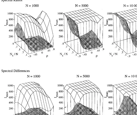
We rst illustrate the performance of the method in terms of overall identication ability. LetImaxdenote
the number of times (out of the 1000 replications) that the driving frequency yielded the largest spectral ratio (or dierence) among the 51 frequencies eval-uated. Fig. 1 graphs the results of our experiment when the driving frequency f= 0:1 and amplitude
m= 0:1;0:5 (the shaded surface corresponds to 0.1 and the unshaded corresponds to 0.5) for both spectral ratios and spectral dierences. Each subgraph shows
Imax as a function of the allocation proportionNs=N and the error correlation. From these graphs, we see that spectral ratios have the greatest power (i.e., the highest probability of correctly detecting the model term) forfar from zero, and spectral dierences have
the greatest power fornear zero. As expected, the power increases as the sample sizeN increases or as the amplitude of the factor level increases. Graphs for
f= 0:4 (not shown) essentially reect the curves of Fig. 1 around= 0.
The allocation proportion clearly aects the power of both spectral tests, although the results are most readily apparent for the case m= 0:1. For the most part, the screening power is the lowest atNs=N= 0:1; the power increases as Ns=N increases to 0.7. Any further increase in Ns=N results in lower or equal spectral power for the spectral ratio approach, while the power increases slightly for some of the spectral dierence experiments. Similar gures result when the driving frequency is changed. Thus, it appears that identication can be improved for small-sample FDEs by allocating more than half of the data to the signal run.
We also consider the performance on an individual experiment basis by examining the number of identi-cations as functions of the data allocation and spec-tral frequency for a subgroup of the design points:
N= 1000 or 5000; = 0:7 andf= 0:1. We use this subgroup for illustration because, as Fig. 1 indicates, neither spectral approach does a good job of correctly identifying the indicator frequency across all alloca-tion proporalloca-tions and both values ofm. When spectral ratios are used, then for low N and low m the fre-quencies most likely to be associated with the highest spectral ratio are 0.0 and 0.5: the indicator frequency is not selected particularly more than any of the other frequencies, although the correspondingImaxis lowest
forNs=N= 0:1. As the sample size increases, the indi-cator frequency is much more likely to yield the largest spike: only the frequency of 0.5 also stands out against the background noise. For the larger value ofm, the indicator frequency is chosen most often. Neighbor-ing frequencies occasionally yield larger spectral ra-tios for smallNs=N, due to a phenomenon known as the smearing of the spectrum. A pattern of screen-ing power that increases sharply and then decreases slightly withNs=Noccurs forN= 1000; the procedure correctly identies the indicator frequency in all cases forNs=N¿0:3 whenN= 5000.
Fig. 1. Correct identications for autoregressive system, amplitudem= 0:1 (shaded) andm= 0:5 (unshaded).
spike. This occurs, regardless of the driving fre-quency, because the noise spectrum is skewed right ( ¿0). If ¡0, then the false positives are clus-tered around frequencies near 0.5 rather than those near zero. However, consistent with Fig. 1, the iden-tication power increases and then stabilizes asNs=N increases.
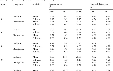
A more detailed look at the performance is provided in Table 1, in which terms have been averaged over runs with non-identical factors in order to reduce the impact of inherent system characteristics. To construct this table we begin, for every one of the 600 design
Table 1
Average magnitudes of spectral terms for autoregressive system
Ns=N Frequency Statistic Spectral ratios Spectral dierences
N N
1000 5000 10 000 1000 5000 10 000
Indicator Mean 4.54 8.43 11.29 0.31 0.69 0.97
0.1 Std. dev. 1.92 2.02 2.15 0.24 0.21 0.20
Background Mean 1.23 1.10 1.04 −0:00 0.00 −0:00
Std. dev. 0.72 0.41 0.33 0.20 0.13 0.11
Indicator Mean 7.06 13.91 19.01 0.53 1.20 1.70
0.3 Std. dev. 2.64 3.08 3.43 0.23 0.20 0.19
Background Mean 1.21 1.03 1.03 0.01 −0:00 −0:00
Std. dev. 0.60 0.34 0.28 0.16 0.11 0.09
Indicator Mean 9.12 17.84 24.40 0.69 1.55 2.19
0.5 Std. dev. 3.51 4.13 4.66 0.22 0.20 0.19
Background Mean 1.20 1.05 1.03 0.01 0.00 −0:00
Std. dev. 0.60 0.33 0.27 0.16 0.11 0.09
Indicator Mean 11.00 21.16 28.88 0.82 1.83 2.59
0.7 Std. dev. 5.05 5.55 6.17 0.23 0.20 0.19
Background Mean 1.22 1.07 1.05 0.01 0.00 0.00
Std. dev. 0.66 0.36 0.29 0.16 0.11 0.09
Indicator Mean 14.67 25.17 33.77 0.93 2.08 2.94
0.9 Std. dev. 18.33 8.99 9.68 0.25 0.21 0.20
Background Mean 1.42 1.12 1.09 0.02 0.00 0.00
Std. dev. 2.90 0.47 0.37 0.20 0.13 0.11
Because the term associated with the indicator frequency may be selected as important even if it does not yield the largest spectral ratio (or dier-ence), Table 1 provides some information about how powerful the screening procedure might be for an unknown (simple) system. For example, the mean spectral ratio associated with the indicator frequency is 3.5 times as large as the mean background ratio when N = 1000 and Ns=N = 0:1. When Ns=N in-creases to 0.9 for this value ofN, the mean spectral ratio for the indicator frequency is 10 times as large as the mean background ratio. This improvement (roughly tripling the average spike for the indicator frequency) also holds asNs=N increases from 0.1 to 0.9 for the other two values of N, even though the tests with larger N are initially more powerful. For
N= 10 000, the mean spectral ratio for the indicator is about 11 times as large as the mean background ratio when Ns=N = 0:1, and about 33 times as large
as the mean background ratio whenNs=N= 0:9. The spectral dierences show similar behavior, although the scale is dierent. The average spectral dier-ences for the non-indicator frequencies conform with theory, and are not statistically distinguishable from zero. Increasing the allocation from Ns=N = 0:1 to
Ns=N= 0:9 roughly triples the magnitude of the spike associated with the indicator frequency. This shows that the power of both the spectral ratio and dierence approaches improves as the allocation ratio increases, at least over the range of allocations and sample sizes examined.
3. African tanker example
A port in Africa is used to load tankers with crude oil for overwater shipment, and the port has facil-ities for loading more than one tanker simultane-ously. The tankers are of three dierent types and have dierent service time distributions. All tankers in the harbor require the services of a tug to move into (and later out of) a berth. The tugs have speci-ed priorities for beginning deberthing=berthing ac-tivities, based on their location (harbor, berths), the availability of berths, and the queues of boats requir-ing berthrequir-ing or deberthrequir-ing. The area experiences frequent storms. Tugs will not start new activities when a storm is in progress but will always nish an existing activity. If a tug is traveling from the berths to the harbor without a tanker when a storm begins, it will turn around and head for the berths.
The data collection unit we use is a single week. The performance measure is the average time a ship waits before beginning loading. As before, we investigate the impact of the allocation ratioNs=N, the total sam-ple sizeN, and the driving frequency assignment on the FDE factor screening ability.
3.1. Experimental design
Levels for the eleven factors we examine are given in Table 2. We ran the experiments with three values ofN:N = 5000 (small),N= 10 000 (medium), and
N = 25 000 (large). Three sets of driving frequency assignments (FA1, FA2, and FA3) are also used. Each
factor in FA1is assigned a frequency using Jacobson
et al.’s algorithm [2] and the code provided in [11]. This frequency assignment results in unique iden-tication frequencies for all main eects, quadratic eects, and two-way interactions. The driving fre-quencies are rotated for FA2 and FA3 so that each
factor is oscillated at low, medium, and high fre-quencies during the course of our investigation. Our window size for a particular signal (or noise) run is set to min{2000;Ns−100; (N −Ns)−100}. If the Tukey window [1, p. 114] gives negative estimates for noise runs, then we compute the absolute value of negative signal-to-noise ratios. It took over 13 CPU days on a Pentium 166 to conduct these 45 000 FDEs – 1000 replications for each of the 45 combinations of N, Ns=N, and frequency assignments. (Note that all factor levels are dynamically oscillated within
each replication.) Files containing spectral dierences and spectral ratios amounted to 165 megabytes of summary data.
3.2. Baseline determination
In order to compare and validate FDE factor screen-ing results, we should know the factors with greatest impact on ship waiting time. Unlike the simple autore-gressive system example of Section 3, we do not know the true nature of the underlying response surface. Therefore, we ran several full 311 (177 147 run)
fac-torial experiments. Each of the 177 147 design points corresponds to xing each of the eleven factors at one of three levels. For quantitative factors, these are the low and high levels given in Table 2, as well as the center value 0.5(low level + high level). For the ve qualitative factors (distribution types), the levels correspond to using only distribution 1, only tion 2, and an equally weighted mix of the distribu-tions during the course of a simulation run.
We reran the factorial experiment several times, us-ing run lengths rangus-ing fromN= 100 toN= 10 000. (Shorter run lengths than those needed for frequency domain experiments are possible because the factor levels are xed during the course of each run: it is the between-run performance dierence which indi-cates the presence of signicant factor eects.) Some of the design points appear to be unstable (i.e., large average queue lengths result). Nonetheless, regression models involving eleven main eects, 55 two-way in-teractions, and eleven quadratic eects consistently identify factor 3 (ship interarrival mean), factor 6 (number of berths), and factor 7 (loading time mean) as the most important determinants of ship waiting time, regardless of run length. (R2 ranges from 0.740
to 0.808 for models containing terms involving only these factors, while R2 ≈ 0:813 for the full 77 term models). We thus feel comfortable specifying that a model with terms involving factors 3, 6 and 7 captures the underlying ‘true’ relationship between the factors and the waiting time.
3.3. FDE results
Table 2
Factors and driving frequencies for the African tanker FDE experiments
ID Factor name Type Factor levels Frequency assignmentsa
FA1 FA2 FA3
1 Storm time mean Continuous 3–5 h 1 89 17
2 Storm time distribution Qualitative Uniform=exponential 4 132 29
3 Ship interarrival mean Continuous 8–14 h 10 164 52
4 Ship interarrival distribution Qualitative Uniform=exponential 17 205 67
5 Number of tugs Discrete 1–3 29 1 89
6 Number of berths Discrete 3–5 52 4 132
7 Loading time meanb Continuous shiptype±8 h 67 10 164
8 Loading time distribution Qualitative Uniform=exponential 89 17 205 9 Ship type distribution Qualitative Multinomial with probability vector 132 29 1
{0:5;0:25;0:25}or{0:25;0:25;0:5}
10 Calm time mean Continuous 24 –72 h 164 52 4
11 Calm time distribution Qualitative Uniform=exponential 205 67 10 aDivide entry by 508 to obtainfin cycles=observation.
bshiptypeis 18, 24, and 36 h, respectively, for tankers of type 1, 2, and 3.
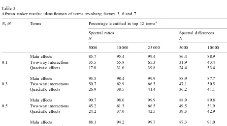
Table 3
African tanker results: identication of terms involving factors 3, 6 and 7
Ns=N Terms Percentage identied in top 12 termsa
Spectral ratios Spectral dierences
N N
5000 10 000 25 000 5000 10 000 25 000
Main eects 85.7 95.4 99.4 86.4 88.9 88.9
0.1 Two-way interactions 35.5 55.8 65.3 31.9 43.4 50.0
Quadratic eects 17.0 31.0 39.8 24.4 33.4 40.1
Main eects 93.5 98.4 99.9 88.9 87.7 92.1
0.3 Two-way interactions 50.7 62.9 66.5 47.1 50.5 53.0
Quadratic eects 26.9 38.5 41.4 36.2 41.1 43.8
Main eects 90.7 98.0 99.9 88.9 89.8 93.6
0.5 Two-way interactions 45.2 61.3 66.5 49.5 51.9 53.7
Quadratic eects 24.2 37.0 42.5 39.3 42.9 44.3
Main eects 88.1 94.2 99.7 87.3 91.0 94.3
0.7 Two-way interactions 41.7 51.9 65.7 50.6 52.5 54.1
Quadratic eects 22.6 28.5 41.8 40.7 43.5 44.4
Main eects 91.0 89.4 91.3 88.4 90.8 93.5
0.9 Two-way interactions 44.3 42.4 45.6 51.3 52.7 54.1
Quadratic eects 24.3 23.6 25.0 41.6 43.9 44.4
for 254 frequencies ({1=508;2=508; : : : ;254=508}) us-ing the fast Fourier transformation code available in [11], spikes corresponding to the 132 indicator fre-quencies (11 each for main and quadratic eects, 110 for interaction terms) are ranked from highest to low-est magnitude. We dene a term to be ‘identied’ for a particular replication if it is among the top 12 spec-tral ratios (or dierences). The entries in Table 3 cor-respond to the percent of time any of the ‘correct’ terms (main, interaction, or quadratic eects involv-ing factors 3, 6 and 7) are among the top 12 indicator frequency spikes in the experiment. Percentage values which dier by more than 2.5 are statistically signi-cant at level= 0:05.
Not surprisingly, in nearly all cases where Ns=N is xed, increasingN increases the percent of terms correctly identied. The exceptions are the alloca-tion Ns=N = 0:9 for spectral ratios, and Ns=N = 0:3 for the main eects using spectral dierences, where there are no statistically signicant increases or de-creases. Thus, additional information generally im-proves the spectral identication. The spectral ratio approach tends to be better at correctly identifying the main eects, while the dierence approach appears better at identifying quadratic terms.
The results also indicate that the data allocation ra-tio aects factor screening. Consider rst the spectral ratio tests. When data are limited (N610 000), the best identication of main eects, two-way interaction eects, or quadratic eects occurs for an allocation
Ns=N= 0:3. However, the impact ofNs=N decreases asN increases to 25 000, unlike our experience with the autoregressive system in Section 2. It appears that if the spectral ratio approach is used for evaluating complex queueing systems, it is better to gain a good estimate of the noise spectrum than to use an equal allocation strategy. The results are not monotonic, so there are limitations on how far this strategy can be extended. Small run lengths for min{Ns; N−Ns}when
N = 5000 and Ns=N 6= 0:5 indicate that the win-dow sizes we use to estimate either the signal (or noise) spectra are less than recommended [11], which may contribute to the degradation in the procedure’s performance.
For the spectral dierence approach, the best alloca-tion strategy is not as consistent. For all three values of
N, the interaction and quadratic terms have the high-est likelihood of appearing among the top 12 terms if
the allocation ratio isNs=N = 0:9. For main eects, an allocation of 0.3 or 0.5 yields the largest observed correct identication percentage whenN= 5000, and an allocation of 0.7 yields the largest results when
N= 10 000 or 25 000, although none of these results are statistically dierent from the 0.9 allocation (at level = 0:05). For xed total sample size N, the best allocation for the ratio approach dominates that of the best allocation for the dierence approach in terms of the correct identication of the three main ef-fects terms, while the dierence approach dominates for identifying the quadratic eects.
The African tanker experiments provide some in-teresting insight into the benets of long noise runs as well, although further work is needed before gen-eralizations can be made. Table 3 shows that if the signal run length is xed, then increasing the length of the noise run improves the screening ability of the spectral ratio approach, though this cannot be said re-garding the spectral dierence approach. For example, compare the spectral ratio cells for{Ns=N= 0:1;N= 25 000}and{Ns=N=0:5;N=5000}. Both are based on signal runs with 2500 observations, yet the detection percentage is signicantly higher (at= 0:05) in the former case for main eects, two-way interactions, and quadratic eects. While we do not have direct comparability of signal run lengths in other situations, there are a total of 14 combinations that can be made with{N′
s6Ns; N′¿ N}. The 42 spectral ratio entries in Table 3 corresponding to the main eects, two-way interactions and quadratic terms for these 14 combina-tions are always greater for{N′
s;N′}than for{Ns;N} and statistically signicant (at = 0:05) in 88% of the cases. In contrast, no clear pattern emerges for the spectral dierence approach. It does appear that if {Ns −Ns′¿1500}, then using {Ns;N} instead of
{N′
s;N′}signicantly increases the correct identica-tion percentage for interacidentica-tion and quadratic terms, although not for main eects.
4. Concluding remarks
be improved by allocating the majority of the data to signal runs (Ns=N ¿0:5). It may be that performance improves further if spectral terms are pooled to form the denominator used in the spectral ratio test, as sug-gested by Morrice and Schruben [5].
At times, the analyst might have baseline results from a previous experiment or (if FDE is used on a real system) historical operating data. If these data are deemed adequate representations of system per-formance, most or all of the new eort could be ex-pended on the signal run. This might be particularly benecial for investigations of complex systems, such as the African tanker problem examined in Section 3. An interesting question is whether or not it would be benecial to use a single noise run for multiple sig-nal runs if more than one sigsig-nal run is to be made, eectively combining the results of three noise runs. In the spectral ratio case, we observe that long noise runs increase the ecacy of the screening procedure, but it is not clear what would be lost by removing the independence across frequency assignments.
Our results also indicate potential pitfalls. The in-vestigation of autoregressive models in Section 2 indi-cates that whenNis small, the spectral ratio method is prone to large (spurious) spikes appearing nearf= 0:5 or f= 0 cycles=observation. Although this behavior is rapidly alleviated as the sample size increases, it suggests that the analyst may wish to avoid frequen-cies close to either endpoint whenN is limited. Since Jacobson et al.’s algorithm [2] always species a fre-quency of the form 1=x for some integer divisor x, the analyst might do better to prompt the procedure fork+ 1 driving frequencies (rather thank) and dis-card this lowest frequency, particularly if only a sin-gle run is to be made. In contrast, false positives for the spectral dierence method appeared to occur over wide bands of frequencies, indicating that this tech-nique may be less suitable for screening purposes if
N is small. An issue that could be addressed in future research is whether or not it is benecial to use both spectral ratios and spectral dierences within a single FDE, since neither method dominates the other over all driving frequencies.
The goal of this paper is to examine the eects of data allocation on the screening capabilities of fre-quency domain experiments, rather than to contrast FDE results with those of conventional experimental designs. Nonetheless, the African tanker results
pro-vide a vivid reminder of the need for this type of screening procedure. It took just under 24 h of CPU time on a Pentium 166 PC to generate the data for the factorial experiment withN = 5000, with many design points indicating an unstable system congu-ration. In contrast, a single replication of an FDE with
N= 25 000 required only 40 CPU seconds.
References
[1] C. Chateld, The Analysis of Time Series, 4th Edition, Chapman & Hall, New York, 1989.
[2] S.H. Jacobson, A.H. Buss, L.W. Schruben, Driving frequency selection for frequency domain simulation experiments, Oper. Res. 39 (6) (1991) 917–924.
[3] A.M. Law, W.D. Kelton, Simulation Modeling and Analysis, 2nd Edition, McGraw-Hill, New York, 1991.
[4] D.J. Morrice, S.H. Jacobson, Amplitude selection in transient sensitivity analysis, in: C. Alexopoulos, K. Kang, W.R. Lilegdon, D. Goldsman (Eds.), Proceedings of the 1995 Winter Simulation Conference, Institute of Electrical and Electronic Engineers, Piscataway, NJ, 1995, pp. 330 –335. [5] D.J. Morrice, L.W. Schruben, Simulation factor screening
using harmonic analysis, Management Sci. 39 (12) (1993) 1459–1476.
[6] A.A.B. Pritsker, Introduction to Simulation and SLAM II, 2nd Edition, Wiley, New York, 1989.
[7] J.K. Robinson, L.W. Schruben, J.W. Fowler, Experimentation with large-scale semiconductor simulations: a frequency domain approach to factor screening, in: D. Mitta, L. Burke, G. Tonkay, J. English, J. Galliamore, G. Klutke (Eds.), Proceedings of the 1993 IIE Research Conference, Institute of Industrial Engineers, Los Angeles, CA, 1993.
[8] P.J. Sanchez, Design and analysis of frequency domain experiments, Ph.D. Dissertation, School of Operations Research and Industrial Engineering, Cornell University, Ithaca, NY, 1987.
[9] P.J. Sanchez, A.H. Buss, A model for frequency domain experiments, in: A. Thesen, H. Grant, W.D. Kelton (Eds.), Proceedings of the 1987 Winter Simulation Conference, Institute of Electrical and Electronic Engineers, Piscataway, NJ, pp. 424 – 427.
[10] P.J. Sanchez, S.M. Sanchez, Design of frequency-domain experiments for discrete-valued factors, Appl. Math. Comput. 42 (1) (1991) 1–21.
[11] S.M. Sanchez, F. Moeeni, P.J. Sanchez, So many factors, so little time: a frequency domain approach for factor screening, Technol. Oper. Rev. (2000), forthcoming.
[12] R.G. Sargent, T.K. Som, Current issues in frequency domain experimentation, Management Sci. 38 (1992) 667–687. [13] T.J. Schriber, Simulation Using GPSS, Wiley, New York,
1974.
![EFEK ANTIFUNGI EKSTRAK ETANOL DAUN RUMPUT MUTIARA (Hedyotis corymbosa [L.] Lamk) TERHADAP PERTUMBUHAN Candida albicans SECARA IN VITRO.](data:image/gif;base64,R0lGODlhAQABAIAAAP///wAAACH5BAEAAAAALAAAAAABAAEAAAICRAEAOw==)