Epistemic considerations of decision making in games
* Mamoru Kaneko
Institute of Policy and Planning Sciences, University of Tsukuba, Ibaraki 305, Japan
Abstract
From the Ex Ante point of view, an axiomatization of decision making in a game with pure strategies is given, while considering its epistemic aspects in propositional game (epistemic) logic. Our axiomatization consists of four base axioms for predicted final decisions. One of them is an epistemic requirement, which together with the others leads to an infinite regress of the knowledge of these axioms. The resulting outcome of this regress is expressed as the common knowledge of the base axioms. We give meta-theoretical evaluations of the derivation of this infinite regress, and consider its implications in solvable and unsolvable games. For a solvable game, it determines predicted decisions to be the common knowledge of a Nash equilibrium, and for an unsolvable game, it is the common knowledge of a subsolution in Nash’s sense. The latter result needs the common knowledge of the additional information of which subsolution would be played. We give also meta-theoretical evaluations of these results. 1999 Elsevier Science B.V. All rights reserved.
Keywords: Game Logic; Infinite regress of knowledge; Common knowledge; Final decisions; Nash equilibrium; Solvable and unsolvable games
1. Game logic approach and meta-theoretic evaluations of some game theoretic considerations
In this paper, decision making in a game is considered from the Ex Ante point of view in an axiomatic manner. For such decision making, players’ knowledge and thinking on the game situation are essential. To describe these epistemic aspects as well as the game situation, we will use the propositional fragment of game logic developed in Kaneko-Nagashima (1996) and (1997a). In the framework of game logic, Kaneko-Kaneko-Nagashima (1991, 1996) presented base axioms for decision making, and showed that these base axioms lead to an infinite regress of the knowledge of the axioms themselves, the result
*Corresponding author.
E-mail address: [email protected] (M. Kaneko)
of which is expressed as the common knowledge of the axioms. Then they solved this infinite regress in the sense that the common knowledge of the axioms determines the final decisions to be the common knowledge of a Nash equilibrium under the common knowledge assumption of interchangeability of Nash equilibria. The objectives of this paper are to evaluate the derivation of the infinite regress in a meta-theoretic manner, which means to consider whether or not a player can prove certain propositions related to the derivation. We also give a full consideration of decision making in an unsolvable game as well as meta-theoretic evaluations of it.
In Ex Ante decision making, since each player makes a strategy choice before the actual play of a game, the knowledge of the structure of the game as well as predictions on the other players’ strategy choices may be needed. In the literature of game theory, the Bayesian approach to this problem has been dominant. In the Bayesian approach, the players’ knowledge is described by means of a subjective probability on possible types of each player, and classical game theory is treated as a trivial case – games with complete information. A game with complete information itself is, however, not trivial in that it has at least the description of the constituents of a game. Although the Bayesian approach has been shown to be quite rich in capturing various economic problems, it is incapable of treating players’ logical and mathematical abilities as well as their knowledge of the descriptions of a game in a direct manner. This leads us to the development of the game logic framework.
Kaneko-Nagashima (1996) and (1997a) developed a hierarchy of logics, GL , GL ,...,0 1 GL ,... ; and GL , where the nesting depths of the knowledge of players’ logical andm v introspective abilities are bounded by m in GL , and they are unbounded in GL . Theym v are predicate logics for the purpose of describing real number theory in its scope, since classical game theory often relies upon real number theory. They are also infinitary to discuss common knowledge, but the limit logic GL is required for the full discussion ofv the problem of common knowledge. The objectives of Kaneko-Nagashima, (1996) and (1997a) were to develop the new framework and to show some possible applications. The purpose of this paper is to give fuller discussions on the epistemic axiomatization of the Ex Ante decision making in a game. For this purpose, we confine ourselves to finite games with pure strategies, for which the propositional fragment of GLv suffices, but any GLm (m , v ) is insufficient for our arguments.
Now we describe our game theoretical problems. We meet two kinds of basic problems arising in the Ex Ante decision making:
(i): solution-theoretic problems; (ii): existence-playability problems.
The first is the problem of how strategy choices are made; and the other is the existence and playability of the solution concept obtained in (i). These problems interact with each other. In this paper, we give the solution-theoretic consideration of the Ex Ante decision making problem for a finite game with pure strategies, and will give also some results on the playability problem.
allow mixed strategies, existence is obtained, but some form of real number theory is involved and is assumed to be known to players, which is a stringent requirement. If a game has a Nash equilibrium in pure strategies, playability is not so serious as in the case with mixed strategies, though some playability problems may remain for such a game. From the viewpoint of playability, the cases with and without mixed strategies are totally different. From the solution-theoretic point of view, however, they do not make much differences. The solution-theoretic considerations given in this paper can be carried over to the case with mixed strategies. The existence-playability of a game with mixed strategies is discussed fully in Kaneko (1997a). In this paper, we restrict our attention to games with pure strategies, which enables us to use the propositional fragment of game logic.
A merit of the game logic approach is not only to describe the epistemic aspects of decision making in an explicit manner, but also to enables us to evaluate such descriptions and resulting outcomes from them in a meta-theoretic manner, that is, we can evaluate what the players can or cannot prove. The undecidability result given in Kaneko-Nagashima (1996), that the existence of a unique Nash equilibrium is common knowledge (in mixed strategies) but the players cannot know what the Nash equilibrium is specifically, is an example of such meta-theoretical evaluations. The main contribu-tions of this paper are meta-theoretical evaluacontribu-tions of the axiomatization and of the resulting outcomes from it.
Our axiomatization consists of four base axioms for predicted final decisions:
D1: Best Response to Predicted Decisions – each player’s decision is a best response to his predictions on the other players’ decisions;
D2: Identical Predictions – each has identical predictions;
D3: Knowledge of Predictions – each knows his own decision and predictions; D4: Interchangeability of Predicted Decisions – each treats the players as in-dependent decision makers.
The first two axioms simply induce Nash equilibrium, but they together with the third and fourth axioms go much further. The third is an epistemic requirement, and the fourth is a requirement of independent decision making. These two additional requirements differentiate substantially our theory from classical Nash equilibrium theory.
The third axiom together with the second leads to an infinite regress of the knowledge of these four axioms, the result of which is expressed as the common knowledge of those axioms. We will evaluate this derivation in a meta-theoretical manner. The evaluation states that to complete the axiomatization, we meet necessarily the infinite regress. The introduction of an epistemic structure also enables us to demarcate playability from the mere knowledge of the existence of a Nash equilibrium, which will be discussed in Subsection 5.2. One result differentiates the case where the players have abstract knowledge of a game from the case where they have the concrete knowledge of it.
common knowledge of a subsolution, which is defined also by Nash himself. In this case, the players need to share some information of which subsolution would or not be played. We will prove that without such additional information, the game is not playable. Here we emphasize that although Nash equilibrium plays a central role in our axiomatic consideration, our concern is individual decision-making in a game situation but not an axiomatization of Nash equilibrium. From this point of view, the fourth axiom is indispensable and plays a crucial role in our considerations. In Section 7, the role of each axiom in our axiomatization is considered.
Our axiomatization looks related to Johansen’s (1982) informal argument on Nash equilibrium. The seemingly self-referential nature of his argument may be regarded as corresponding to our infinite regress of the base axioms. His claim that his postulates determine a Nash equilibrium for a game with a unique Nash equilibrium is consistent with our results. In this paper, however, we will consider epistemic aspects explicitly and also treat unsolvable games. The comparison between his and ours will be given in Subsection 7.2. This paper is related also to Aumann-Brandenberger (1995) in its objectives. These authors considered some epistemic conditions for Nash equilibrium in a Bayesian framework. The difference is that they concern necessary conditions for Nash equilibrium, while our concern is the complete characterization of predicted final decisions with meta-theoretical evaluations (the direct comparisons are difficult since the
1 frameworks are different).
As already stated, the logic GL we use is a propositional fragment of game logic ofv Kaneko-Nagashima (1996) and (1997a). In fact, it is shown in Kaneko (1996) that common knowledge logic developed in Halpern-Moses (1992) and Lismont-Mongin (1994) can be faithfully embedded into our logic (with a slight restriction on our logic). This implies that the results obtained in this paper are all translated into common knowledge logic.
A final remark on GL is that we assume the Veridicality Axiom T :K (A).A, while
v i i
Axiom D :i¬K (i¬A∧A) is adopted in Kaneko-Nagashima, (1996) and (1997a). Thus, we adopt here the S4-type game logic for our presentational purposes, instead of the KD4-type game logic of Kaneko-Nagashima, (1996) and (1997a). However, since the S4-type logic can be faithfully embedded into the KD4-type game logic, the whole argument of this paper can be done in the KD4-type. Finally, we remark that we do not need Axiom 5 : ¬K (A).K (¬K (A)), called the Negative Introspection, which is often
i i i i
an obstacle for proof-theoretic arguments.
We will repeat some results given in Kaneko-Nagashima (1991) and (1996), but give proofs to some of them for completeness. We distinguish the results already given by
*
putting from new ones.
1
2. Preliminaries
In Subsection 2.1 we give basic game theoretical concepts in the nonformalized v
language, and in Subsection 2.2, we give formalized language3 and game logic GL . v In Subsection 2.3, we redescribe game theoretical concepts in the formalized language
v 3 .
2.1. Game theoretical concepts in the nonformalized language
Consider an n-person finite noncooperative game g in strategic form. The players are denoted by 1,...,n, and each player i has, pure strategies with (, $ 2). We assume that
i i
the players do not play mixed strategies. Player i’s strategy space is denoted byS : 5i
hs ,...,si 1 i,ij, and his payoff function is a real-valued function g oni S : 5 S 3 ? ? ? 3 S1 n
for i 5 1,...,n. We call an element in S a strategy profile.
A strategy profile a 5 (a ,...,a ) is called a Nash equilibrium iff for i 5 1,...,n,1 n
g (a) $ g (b ;a ) for all b[S , where a 5 (a ,...,a ,a ,...,a ) and (b ;a ) 5
i i i 2 i i i 2 i 1 i 2 1 i 1 1 n i 2 i
(a ,...,a1 i 2 1,b ,ai i 1 1,...,a ). We denote the set of Nash equilibria of game g by E .n g
Consider a maximal nonempty subset E of E which satisfies the interchangeabilityg
condition:
a,b[E and i 5 1,...,n imply (a ;b )[E. (2.1)
i 2 i
1 n 1 n
This is equivalent to that a ,...,a [E implies (a ,...,a )[E, which states that if each
1 n
i 1 n
player i independently chooses his equilibrium strategy a , the resulting profile (a ,...,a )i 1 n
is also an equilibrium. We call such a maximal set a subsolution, which was introduced by Nash (1951). Each Nash equilibrium belongs to at least one subsolution. We denote
1 s
the subsolutions of game g by E ,...,E . We stipulate that when E is empty,g g g s 5 0. 2
When E is nonempty,g s $ 1. When s 5 1, game g is said to be solvable. 1 2
The game (Battle of the Sexes) of Table 1 has E 5 E <E 5 h(s ,s )j<
g g g 11 21
h(s ,s )12 22 j, and is not solvable. The game of Table 2 is not solvable either and has 1 2
E 5 E <E 5 h(s ,s ),(s ,s )j< h(s ,s ),(s ,s )j. Here (s ,s ) belongs to both
g g g 11 21 11 22 11 21 12 21 11 21
Table 1
s21 s22
*
s11 (2,1) (0,0)
*
s12 (0,0) (1,2)
2
Table 2
s21 s22
* *
s11 (2,2) (1,2)
*
s12 (2,1) (0,0)
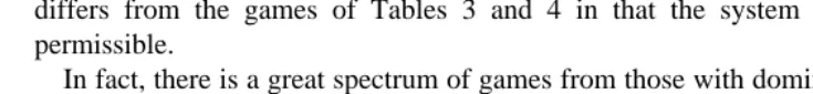
subsolutions. The games of Tables 3 (Prisoner’s Dilemma) and 4 have the same equilibrium sets E 5g h(s ,s )12 22 jand are solvable.
In the next subsection, we give a formal logic in which a game as well as such other epistemic constituents are described.
2.2. Game logic GLv
In the following, we use some notions of predicate logic. Since, however, we use neither variables nor quantifiers, the following logic is essentially propositional.
We start with the following list of symbols:
constant symbols: s ,...,s11 1,; s ,...,s21 2,; ...; s ,...,sn1 n, ;
1 2 n
binary predicate symbols: 5 ; 2n –ary predicate symbols: R ,...,R ;1 n
n-ary predicate symbols: D ,....,D ;1 n
knowledge operator symbols: K ,...,K ;1 n
logical connectives: ¬(not),.(implies),n(and),k(or) ;
parentheses: ( , ).
As in Subsection 2.1, the constants s ,...,s11 1,1; s ,...,s21 2,2; ...; s ,...,sn1 n,n are the players’ strategies. The binary predicate symbol 5 is intended to describe identity between strategies for each single player. The 2n-ary symbol R ( ?: ? ) is used to describei
player i’s payoff function g . The n-ary symbol D ( ? ) is to describe i’s prediction of thei i
players’ strategy choices, that is, D (a ,...,a ) means that i predicts that 1,...,n couldi 1 n
choose a ,...,a as final decisions in their ex ante decision making. Of course, a itself is1 n i
i’s own possible decision. These D ,...,D will be determined by the nonlogical axioms1 n
which will be given in Section 3. By the expression K (A), we mean that player i knowsi
a formula A.
Table 3
s21 s22
s11 (5,5) (1,6)
*
s12 (6,1) (3,3)
Table 4
s21 s22
s11 (5,5) (1,2)
*
First, we develop the space of formulae. For any strategies a ,b inj j S (a and b mayj j j
be identical and j 5 1,...,n), (a 5 b ) is an atomic formula, and for strategy profilesj j
(a ,...,a ),(b ,...,b ) in1 n 1 n S , the expressions R (a ,...,a :b ,...,b ) and D (a ,...,a ) (i 5i 1 n 1 n i 1 n
1,...,n) are also atomic formulae. These atomic formulae correspond to propositional variables in the standard formulation of propositional logic. Since the number of strategies is finite, so is the number of atomic formulae.
0
Let 3 be the set of all formulae generated by the standard finitary inductive 0 definition with respect to ¬,. and K ,...,K from the atomic formulae. That is, 3 is
1 n
the set of 0-formulae defined by the following induction: (0-i): any atomic formula is a 0-formula;
3 (0-ii): if A and B are 0-formulae, so are (¬A),(A.B ) and K (A).
i
k 2 1 k
Suppose that the set3 of (k 2 1)-formulae is already defined (k 5 1,...). Then3 is the set of k-formulae defined by the following induction:
k 2 1
(k-i): any expression in3 <h(nF ),(kF ):F is a nonempty countable subset of
k 2 1
3 jis a k-formula;
(k-ii): if A and B are k-formulae, so are (¬A),(A.B ) and K (A).
i
k v v
We denote
<
3 by 3 . An expression in3 is called simply a formula. Wek , v
abbreviatenhA,BjandkhA,Bjas AnB and AkB, and (A.B )n(B.A) as A;B. We
also abbreviate some parentheses in the standard manner. Also, we callF an allowable
k
set iffF is a nonempty countable subset of3 for some k , v . We say that a formula A is nonepistemic iff it contains no K ,i 5 1,...,n.i
The primary reason for our infinitary language is to express common knowledge explicitly as a conjunctive formula. The common knowledge of a formula A is defined as follows: For any m $ 0, we denote the set hK K ...K : each K is one of K ,...,K andi1 i2 im it 1 n
it±it 1 1 for t 5 1,...,m 2 1jbyK(m). We assume thatK(0) consists of the null symbol e (i.e., e(A) is A itself for any A). We define the common knowledge formula of A as
∧
H
K(A):K[<
K(m)J
, (2.2)m , v
k 2 1
which we denote by C(A). If A is in 3 , the set hK(A):K[
<
m , v K(m)j is ak 2 1 k
countable subset of3 , and its conjunction, C(A), belongs to3 by (k-i). Hence the v
space 3 is closed with respect to the operation C( ? ).
Note that A itself is included as a conjunct in C(A), since K(0) 5 hej. In this sense, C(A) is ‘‘common knowledge’’ instead of ‘‘common belief’’ which is defined to be the conjunction obtained from (2.2) by excluding A.
Base logic GL is defined by the following five axiom schemata and three inference0 rules: for any formulae A,B,C and allowable set F ,
(L1): A.(B.A);
(L2): (A.(B.C )).((A.B ).(A.C ));
(L3): (¬A.¬B ).((¬A.B ).A);
(L4): nF .A, where A[F ;
3
(L5): A.kF , where A[F ;
A.B A
] ] ] (MP) B
hA.B:B[F j
] ] ] ] ] (∧-Rule) A.nF
hA.B:A[F j
] ] ] ] ] (∨-Rule). kF .B
These axioms and inference rules determine base logic GL .0
We define game logic GLv by adding the following axiom schemata and inference rule to GL : for any formulae A,B and i 5 1,...,n;0
(MP ): K (A.B )nK (A).K (B );
i i i i
(T ): K (A).A;
i i
(PI ): K (A).K K (A);
i i i i
(C-Barcan): ∧
H
K K(A):K[<
K(m)J
.K C(A);i i
m , v and
A ] ] (Necessitation): .
K (A)i
We will abbreviate Necessitation as Nec, and use MP , T , PI as generic names fori i i
those for different i.
A proof P in GLv is a countable tree with the following properties: (i) every path from the root is finite; (ii) a formula is associated with each node, and the formula associated with each leaf is an instance of the axioms; and (iii) adjoining nodes together with their associated formulae form an instance of the above inferences. We write£ A
v v iff there is a proof P such that A is associated with the root. For any subsetG of3 , we
4
writeG£ A iff£ ∧F .A for some nonempty finite subsetF of G. When G is empty,
v v
G£ A is assumed to be £ A itself. We also abbreviate G<Q£ A and G<hBj£ A as
v v v v
G,Q£ A andG,B£ A, etc.
v v
When we restrict the use of axioms and inference rules to those of GL , we denote the0 provability relation by £ . Logic GL is an infinitary extension of classical finitary
0 0
propositional logic.
We will use the following facts without references (see Kaneko-Nagashima (1996)).
Lemma 2.1. Let G,Q be sets of formulae, and F an allowable set of formulae. Then
5. £ kK (F ).K (kF ).
v i i
Note that (1)–(3) hold also for £ .
0
Axiom MP and inference rule Nec in addition to GLi 0 give the complete logical ability to each player (see (Kaneko and Nagashima, 1996)). Axiom T , which is calledi
Veridicality Axiom, states that if i knows A, then A is true from the objective point of view. Axiom PI , called the Positive Introspection, means that if player i knows A, hei
knows that he knows A. In fact, these logical and introspective abilities of the players are common knowledge in GL (see (Kaneko and Nagashima, 1996)).v
Axiom C-Barcan is called the common knowledge Barcan axiom. For the development of our framework, C-Barcan will be used to derive the property:
£ C(A).K C(A) for i 5 1,...,n. (2.3)
v i
That is, if A is common knowledge, then each player i knows that it is common knowledge. This property will play an important role in the epistemic axiomatization of final decisions in later sections.
*
Proof of (2.3). . Let K be an arbitrary element in
<
m , v K(m). When K is not theioutermost symbol of K, we have £ C(A).K K(A) by L4. When K is the outermost
v i i
symbol of K, we have £ K(A).K K(A) by PI . This together with £ C(A).K(A)
v i i v
implies £vC(A).K K(A). Thusi £vC(A).K K(A) for all Ki [
<
m , v K(m). Hence£vC(A).nhK K(A): Ki [
<
m , v K(m)j by n-Rule. By C-Barcan, we obtain£ C(A).K C(A). h
v i
Since the finitary propositional modal logic defined by MP , T , PI and Nec in additioni i i
to classical propositional logic is called S4, our logic is an infinitary extension of multi-modal S4 with C-Barcan. Kaneko-Nagashima (1996) and (1997a) assumed the following weaker axiom:
('):¬K (¬A∧A);
i i
instead of Axiom T . Axiom ' is called D in the literature of modal logic. Hence
i i
Kaneko-Nagashima (1996) and (1997a) developed the KD4-type game logic. In the KD4-type game logic, since knowledge is not necessarily objectively true, it is called belief. In fact, knowledge and belief are more fully discussed in the KD4-type game logic. However, we do not treat our subjects in the way that the difference in them is reflected. From the viewpoint of presentational purposes, the S4-type game logic is more convenient than the KD4-type. Hence we adopt the S4-type game logic.
In the subsequent analysis, the relation between the provabilities of GL and GL isv 0 important. For this purpose, we introduce the following notion. Let A be a formula in
v
3 . Then «A is the formula obtained from A by eliminating all the occurrences of
K ,...,K in A, and«G is the set h«A: A[Gj for any setG of formulae. Formula «A is
1 n
nonepistemic, and if A is nonepistemic, «A is A itself. For example, «(K (A)nK (A.
i i
B ).K (B )) is«An(«A.«B).«B, and «(K (A).A)) is («A.«A). For every instance
i i
A of the epistemic axioms,«A is a nonepistemic provable formula with respect to£ and
every instance of Nec becomes a trivial inference with an application of «. This is the reason for Lemma 2.2.(1). We have also the other lemmas (see Kaneko-Nagashima (1996)).
Lemma 2.2.
1. If G£ A, then«G£ «A.
v 0
2. If G£ A or G£ A, then C(G)£ C(A), where C(G) 5 hC(B ):B[Gj.
0 v v
Lemma 2.3.
1. £ C(A.B ).sC(A).C(B ) ;d
v
2. if C(G)£ A, then C(G)£ K (A) for i 5 1,...,n.
v v i
Lemma 2.4. Let F be an allowable set of formulae. Then
1. £vC(nF ).nC(F ), and if F is a finite set, then £vC(nF );nC(F ); 2. £vkC(F ).C(kF ).
Although our analysis is primarily syntactical, we will use some semantic methods in several places. For this purpose, we prepare some semantics and review some results to be used for the subsequent analysis. We say that a formula A is finitary iff it contains no infinitary conjunction and no infinitary disjunctions. We denote the set of all
nonepis-f f
temic finitary formulae by3 . The space3 is closed with respect to¬, . and finitary
f
n,k. When we restrict the language of base logic GL to 3 , the resulting logic is 0
f
classical propositional logic, which we denote by GL . Base logic GL is a conservative0 0
f f
extension of GL , i.e., for any A[3 , 0
f
if£ A, then£ A, (2.4)
0 0
f f
where£ is the provability relation of GL . Of course, the converse of (2.4) holds.
0 0
f
We will use the classical two-valued semantics for GL . An assignment0 t is a function from the set of atomic formulae tohtrue,falsej. We define the truth relation*t relative to
v 2.3. Game theoretical concepts in the formalized language 3
v Now we describe the game theoretical concepts given in Subsection 2.1 in 3 . First, we make the following axiom: for all distinct a ,b [S (i 5 1,...,n),
i i i
Axiom (Eq). a 5 a andi i ¬(a 5 b ).i i
We denote the set of instances of this axiom by Eq, which is a finite set of formulae. Second, we describe the payoff functions g ,..., g in terms of symbols R ,...,R as1 n 1 n
follows: for strategy profiles a,b,a9,b9 with g (a) $ g (b) and g (a9) , g (b9) and i 5i i i i
1,...,n,
Axiom (G ). R (a;b) andg i ¬R (a9;b9).i
We denote by Gg the set of all instances of this axiom. This describes the payoff functions g ,..., g by preferences R ,...,R . It holds that for any a,b[S , either G
extensional definition of a subsolution in our formal language. We denote the following
k
formula by Sol (a):
n
k
S
na 5 yi iD
(2.10)k i 5 1 y[Eg
k k
for k 5 1,...,s . The formula Sol (a) describes ‘‘a belongs to the subsolution E ’’.g
Lemma 2.5.
E
1. Eq,G £ ∧
s
Nash(x);Nash (x) ;d
g 0 x[S
s k
2. Eq,G £ ∧
s
Nash(x);∨ Sol (x) .d
g 0 x k 5 1
We abbreviate ∧x[S as ∧x, etc. unless it is confusing.
Proof. We prove (1). Let a be an arbitrary profile. Suppose G £ Nash(a). Then a[E
g 0 g
E
by (2.8). Thus Eq£ ∨ s∧ a 5 y , i.e., Eqd £ Nash (a). Since Nash(a) is decidable
0 y[Eg i i i 0
E E
under G by (2.7), we have proved Eq,G £ Nash(a). Nash (a). Noting that Nash (a)
g g 0
E
is decidable under Eq, we can repeat a similar argument to have Eq,G £ Nash (a).
g 0
E
Nash(a). Thus Eq,G £ Nash (a);Nash(a). Since a is an arbitrary profile, we have
g 0
E
Eq,G £ ∧
s
Nash(x);Nash (x) .d
hg 0 x
In Section 6, we need to assume that these equivalences are common knowledge among the players. If we assume that Axioms Eq and Gg are common knowledge, these equivalences are common knowledge, particularly, (2) becomes
s
k
C(Eq),C(G )£ nC Nash(x)
S
;k Sol (x) .D
(2.11)g v x
k 5 1
This follows from Lemmas 2.5, 2.2.(2), 2.3.(1), and 2.4.(1). Note, however, that the
E s k
common knowledge of the equivalence of Nash (a) and ∨k 5 1Sol (a) is provable
E s k
without these axioms. Indeed, £ Nash (a); ∨ Sol (a) for all a[S , which this is
0 k 5 1
E s k
simply extensional equivalence, and then £ ∧ C Nash (x)
s
;∨ Sol (x) .d
v x k 5 1
Note that Axioms Eq and G are consistent with respect to£ , i.e., there is no formula
g 0
A such that Eq,G £ ¬AnA. This can be proved by constructing a model of them by the
g 0
f
Soundness Theorem for GL . It follow from this that C(Eq) and C(G ) are also0 g
consistent with respect to£ by Lemma 2.2.(1), which we will use in Sections 5 and 6.
v
3. Final decision axioms
In a given game g, each player deliberates on his and the others’ strategy choices and may reach some predictions on their final decisions. Now we describe these ‘‘predic-tions’’ by n-ary symbols D ,...,D , that is, each D (a ,...,a ) is intended to mean that1 n i 1 n
player i predicts that players 1,...,n could choose (a ,...,a ) as their final decisions, where1 n
The following are base axioms for D ( ? ),...,D ( ? ): for each i 5 1,...,n,1 n
0
Axiom D1 . ∧ D (x). ∧ R (x:y ;x ) ;
i x
s
i yi i i 2 id
0
Axiom D2 . ∧ ∧
s
D (x).D (x) ;d
i x j i j
0
Axiom D3 . ∧ sD (x).K (D (x)) ;d
i x i i i
0
Axiom D4 . ∧ ∧ ∧
s
D (x)nD ( y).D (x ; y ) .d
i x y j i i i j 2 j
These are verbally as follows:
0
D1 : (Best Response to Predicted Decisions): If player i predicts final decisionsi
x ,...,x for the players, then his own final decision x maximizes his payoff against his1 n i
prediction x , that is, x is a best response to x .2 i i 2 i 0
D2 : (Identical Predictions): The other players reach the same predictions as playeri
i’s. 0
D3 : (Knowledge of Predictions): Player i knows his own predictions.i
0
D4 : (Interchangeability): In predicting the players’ decisions, he assumes that thei
players are independent decision makers. This axiom states that when multiple predictions are possible, any combination of predictions on individual decisions is again a prediction profile. This may be better understood by looking at the equivalent formulation focussing on individual predictions (see Subsection 7.2).
These axioms are requirements for decision (prediction) making in the mind of each player i 5 1,...,n. Hence we assume that these axioms are known to player i. These are
0 0 0 0
described as K (D1 ), K (D2 ), K (D3 ), K (D4 ). We denote these formulae by D1 ,i i i i i i i i i
D2 , D3 , D4 , respectively. Now, the problem is whether these axioms determinei i i
‘‘unknown’’ symbol D ( ? ) in terms of the ‘‘primitives’’, s ,...,si 11 1,1; ...; s ,...,sn1 n,n, 0 0
R ,...,R and K ,...,K . In the following, we denote D11 n 1 n i ∧...∧D4 and D1i i∧...∧D4 byi
0
D (1–4) and D (1–4).i i
We will take three steps to distil ‘‘solutions’’ from these axioms. Since the three steps are quite different, we give a brief explanation of these steps.
Step 0. The knowledge, D (1–4), of the base axioms is incomplete as the requirement toi
determine D ( ? )’s, and the process of completing this knowledge forms an infinitei
regress of the knowledge of D (1–4),...,D (1–4). The resulting outcome of this infinite1 n
regress is described as the common knowledge of D (1–4),...,D (1–4), which we will1 n
denote by C(D(1–4)).
verify that the solutions obtained satisfies the equation. In the same way, we have two steps to solve the common knowledge of the axioms as follows:
Step 1. We derive a necessary condition from the common knowledge C(D(1–4)) of the above axioms. In Section 4, we will discuss Steps 0 and 1.
Step 2. We will verify that the necessary condition derived in Step 1 is a solution for C(D(1–4)). In fact, this depends upon a game. In Section 5, we will treat games satisfying interchangeability (2.1). In Section 6, we consider games not satisfying (2.1), where some additional information is required to have a ‘‘solution’’.
In addition to these three steps, we will discuss, in Section 7, the status of each of the above base axioms in our axiomatization, their variants and the comparisons of Johansen (1982).
In the remaining of this section, we prepare some basic results on the axioms D (1–4), ..., D (1–4).1 n
Notice that D ( ? )’s occur in Axiom D2 for all j. These D ( ? )’s are determined by thej i j
other axioms D (1–4)’s. Then D ( ? )’s would be just symbols without meaning forj j
player i unless he knows the other axioms D (1–4)’s ( j±i ). In other words, D (1–4)’s
j j
give operational meanings to the symbols D ( ? )’s. We need to give some operationalj
knowledge of D ( ? )’, which is assumed here to be D (1–4)’s. In fact, this is the first stepj j
to the infinite regress to be discussed later.
The following proposition states that the addition of D (1–4)’s to D (1–4) isj i
nontrivial.
Proposition 3.1. Let i, j be distinct players. Then
0 0
1. neither D (1–4)£ D (1–4) nor D (1–4)£ ¬D (1–4);
i v j i v j
2. neither D (1–4)£ D (1–4) nor D (1–4)£ ¬D (1–4);
i v j i v j
3. neither D (1–4)£ K (D (1–4)) nor D (1–4)£ ¬K (D (1–4)).
i v i j i v i j
Proof. We prove only the first assertion of (3). Suppose D (1–4)£ K (D (1–4)), i.e.,
i v i j
£ D (1–4).K (D (1–4)). By Lemma 2.2.(1), £ «D (1–4).«K (D (1–4)), which
v i i j 0 i i j
0 0
implies £ D (1,2,4) . D (1,2,4), since «D3 is equivalent to ∧ sD (x).D (x) .d
0 i j k x k k
0 0 f
Hence * D (1,2,4). D (1,2,4) for any assignment t by Soundness for GL .
t i j 0
0
However, we can construct an assignment t0 so that *t0D (1,2,4) but noti
0
* D (1,2,4), a contradiction. Therefore it is not the case that D (1–4)£ K (D (1–
t0 j i v i j
4)). h
We denote ∧jD (1–4) by D(1–4). Proposition 3.1 implies that for D ( ? )’s to bej j
meaningful in Axiom D2 , we need to assume K (D(1–4)). In fact, these are stilli i
insufficient to determine the meanings of all D ( ? )’s in K (D(1–4)), which will bej i
discussed in Section 4. Here we state only the following undecidability:
neither D(1–4)£ K D(1–4) nor D(1–4)s d £ ¬K D(1–4) .s d (3.1)
That is, the knowledge of D(1–4) is not derived from D(1–4) itself. In Section 4, we will give a general version of this claim, which leads to the infinite regress of the knowledge of D(1–4). The resulting outcome of this infinite regress would be expressed as the common knowledge of D(1–4).
0 0
In the following, we denote ∧jDtj and ∧jDt by Dt and Dt for t 5 1,2,3,4, andj
0 0 0
D1 ∧D2 and D1∧D2nD4 by D (1,2) and D(1,2,4), etc.
0
Lemma 3.2. D (1,2)£ ∧ sD (x).Nash(x) .d
0 x i
0 0
Proof. Let a be an arbitrary profile. Since D2 £ D (a).D (a) and D1 £ D (a).
0 i j 0 j
0
∧ R (a ;a :y ;a ) for all i, j, we have D (1,2)£ D (a).∧ R (a ;a :y ;a ) for all j.
yj j j 2 j j 2 j 0 i yj j j 2 j j 2 j
0 0
Thus D (1,2)£ D (a). ∧ ∧ R (a ;a :y ;a ) by ∧-Rule, i.e., D (1,2)£ D (a).
0 i j yj j j 2 j j 2 j 0 i
Nash(a). Hence we have the assertion. h
0
Thus, Nash equilibrium is a necessary condition for Axioms D (1,2). In fact, we will show in our full axiomatization that D (a) implies C(Nash(a)), i.e., it is the commoni
knowledge that a is a Nash equilibrium. The following lemma is indicative of this common knowledge result.
Lemma 3.3. D(2,3)£ ∧
s
D (x).K (D (x)) for any i, j,k (i, j,k may be identical ).d
v x j i k
Proof. Let a be an arbitrary profile. Since D2 £vK D (a)s .D (a) , we have D2d
i i k
£vK (D (a)).K (D (a)) by MP and MP. Since D2£ D (a).D (a) and D3 £ D (a).
i i i k i v j i v i
K (D (a)), we have D(2,3)£ D (a).K (D (a)). Hence we have D(2,3)£ D (a).K (D (a)).
i i v j i i v j i k
This implies the assertion. h
We prepare one more lemma, which will be used in the later sections.
Lemma 3.4.
1. «D(1–4) is consistent with respect to £ , and «D(1–4),D (a) is also consistent for
0 i
any a[S .
2. £ D(1–4) does not hold.
v
Proof.
0
1. «D(1–4) is equivalent to D (1,2,4) with respect to £ . To prove the consistency of
0
0 f
D (1,2,4), by Soundness for GL , it suffices to construct an assignment0 t so that 0
*t D (1,2,4). Definet so that t (D (a)) 5 false for all profiles a and i 5 1,...,n. Theni
0
*t D (1,2,4) in the trivial sense. The latter is proved by modifying t . 0
2. Suppose £ D(1–4). Then £ «D(1–4), i.e., £ D (1,2,4), by Lemma 2.2.(1).
How-v 0 0
0
ever, we can constructt in a similar manner as in (1) so that D (1,2,4) is false, which 0
together with (2.4) implies not £ D (1,2,4). Thus £ D(1–4) is not the case. h
4. Infinite regress of the knowledge of the axioms and its evaluations
In this section, we show that the process of making Axioms D1 to D4 meaningful forms an infinite regress of the knowledge of D(1–4). The resulting outcome of this infinite regress is expressed as the common knowledge of D(1–4). We make proof-theoretical evaluations of this infinite regress.
4.1. Infinite regress of the knowledge of the final decision axioms
It could be found by looking at Lemma 3.3 carefully that axioms D1–D4 require each player to know them. Lemma 3.3 states that each player knows any other players’ predictions on final decisions, but this would not make sense unless the meaning of ‘‘predictions on final decisions’’ is given to the players. In fact, the meaning is determined by the above four axioms themselves. Therefore each player needs to know them, i.e., K (D(1–4)) for i 5 1,...,n.i
Once the players know these axioms, each knows the consequences from these axioms such as the assertion of Lemma 3.2, i.e., ∧ K (D(1–4))£ n K D (x)s .Nash(x)) . It is,d
j j v x i i
however, more to the point that the following is provable: for any l,k 5 1,...,n,
nK (D(1–4))£ nsD (x).K K (D (x)) .d (4.1)
j v x i l k i
j
In (4.1), the ‘‘imaginary’’ player k in the mind of player l knows that x is a profile of predicted decisions. This imaginary player k is not given the operational meaning, D(1–4), of ‘‘final decisions’’, though ‘‘real’’ k is assumed to know D(1–4). This means that (4.1) does not make sense for the imaginary k. Thus we need to assume
5
K K (D(1–4)): we reach the assumption setl k hL(D(1–4)): L[
<
t # 2K(t)j. Once we assume this set of axioms, we would again meet the problem parallel to that arose in (4.1), that is, it holds that for any K[K(3),L(D(1–4)): L[
<
K(t) £ n D (x).K(D (x)) .H
J
v x s i i dt # 2
If we assume the knowledge of D(1–4) up depth 2, the knowledge of depth 3 is necessarily involved. The imaginary players in the epistemic world of depth 3 should know D(1–4).
In general, we have the following proposition.
Proposition 4.1. For any players i, j, finite m $ 0 and K[K(m 1 1),
hL(D(2,3)): L[
<
K(t)j£v ns
D (x).K(D (x)) .d
i j
x t # m
5
Proof. Let a be an arbitrary profile. We prove that for any K[K(m 1 1),hL(D(2,3)):L[
<
K(t)j£ D (a).K(D (a)). For m 5 0, this is Lemma 3.3. Now we assume thet # m v i j
9
induction hypothesis that the assertion holds for m. Let K 5 K Kk[K(m 1 2). Then 9
K [K(m 1 1). By the induction basis and some applications of Nec, MP and MP ,i
9 9 9 9
K9(D(2,3))£ K D (a)
s
.K (D (a)) , and then K (D(2,3))d
£ K (D (a)).K K (D (a)). Thisv i k j v i k j
together with the induction hypothesis implieshL(D(2,3)):L[
<
K(t)j£ D (a).t # m 1 1 v i
9
K K (D (a)). h
k j
Thus, if we assume the knowledge of Axiom D(1–4) up to depth m, the knowledge of depth m 1 1 is necessarily involved. Hence the knowledge of D(1–4) up to depth m 1 1 should be added. The following theorem states that this addition is inevitable, which is a general version of (3.1). This will be proved in Subsection 4.2.
Theorem 4.A. For any finite m $ 0 and for any K[
<
t . m K(t),neither
H
L(D(1–4)):L[<
K(t)J
£ K(D(1–4)) (4.2)v
t # m
nor
H
L(D(1–4)):L[<
K(t)J
£ ¬K(D(1–4)). (4.3)v
t # m
This theorem states that without assuming K(D(1–4)) for all K of all depths, some imaginary players living in the mind of the players in some depth could not know the definition of D ( ? )’s. To avoid this problem, we should assumei
hK(D(1–4)):K[
<
K(t)j. (4.4)t , v
Thus we meet an infinite regress of the knowledge of axioms D(1–4). The infinite regress leads to the set of (4.4), and its conjunction is the common knowledge of D(1–4). We will adopt this common knowledge formula as an axiom and consider its implications. The following result holds, which was given in Kaneko-Nagashima (1991) and (1996). For completeness, we will give a brief proof. In the following, when we write D ( ? ),D ( ? ) without quantification of i, j, they are arbitrary players.i j
Proposition 4.2.
1. C(D(2,3))£ ∧
s
D (x).C(D (x)) .d
v x i j
2. C(D(1–3))£ ∧ sD (x).C(Nash(x)) .d
v x i
Proof. (1) follows Proposition 4.1. Consider (2). Let a be an arbitrary profile. First, D(1,2)£ D (a). Nash(a) by Lemma 3.2. Hence, by Lemma 2.2.(1), we have
0 i
C(D(1,2))£ C D (a)s .Nash(a) , and C(D(1,2))d £ C(D (a)).C(Nash(a)) by Lemma
v i v i
2.3.(1). Since C(D(2,3))£ D (a).C(D (a)) by (1), we have C(D(1–3))£ D (a).
v i i v i
In fact, C(Nash(x)) will be shown to be the solution of C(D(1–4)) for a game satisfying interchangeability (2.1), which will be the subject of Section 5. Here, we can ask whether the conclusion of Proposition 4.2.(2) is provable from the knowledge of D(1–4) up to some finite depth. The following theorem states the negative answer. Since this can be proved in the same manner as in the proof of Theorem 4.A, we omit the proof.
Theorem 4.B. For any finite m,
neither
H
L(D(1–4)):L[<
K(t)J
£ nsD (x).C(Nash(x))dv x i t # m
nor
H
L(D(1–4)):L[<
K(t)J
£v¬nsD (x).C(Nash(x)) .di x t # m
The above derivation of the infinite regress, a fortiori, C(D(1–4)), is still heuristic. However, it can be formulated in the following manner, whose proof is also omitted.
Theorem 4.C. LetG be a set of formulae. Suppose that G£ ∨ K(D (x)).K(D(1-4)) for
v x i
all K[
<
K(m). ThenG£ ∨ D (x).C(D(1–4)).m , v v x i
In Subsection 4, we show that this setG needs to contain some common knowledge. The results given in this section are still purely solution-theoretic: they do not require the players to know the game, i.e., neither Axioms Eq nor G . The knowledge of theg
structure of the game will be needed in Sections 5 and 6.
4.2. Evaluations of the infinite regress
To prove the undecidability theorems given in the above subsection, we need the depth d(A) of a formula A. Using this concept, we will evaluate the provability of an epistemic statement.
We define the depthd(A) by induction on the structure of a formula from the inside: (0):d(A) 5 5for any atomic A;
(1):d(¬A) 5 d(A);
(2):d(A.B ) 5 d(A)<d(B);
(3):d(nF ) 5 d(kF ) 5
<
A[Fd(A);h( j )j ifd(A) 5 5
h( j,i ,...,i ):(i ,...,i )[d(A) and j±i j<
(4):d(K (A)) 5j
5
1 m 1 m 1h(i ,...,i ):(i ,...,i )[d(A) and j 5 i j otherwise.
1 m 1 m 1
For any set G of formulae, let d(G) be
<
A[Gd(A). Define supd(G) 5 0suphm:(i ,...,i )[d(G)j. For example, d(D3 ) 5 d(D1 ) 5 h(i )j,d(D3) 5 h(i ):i 5 1,...,nj
1 m i i
andd(∧ K (D(1–4))) 5 h(i, j ):i±jj. i i
proved in the Gentzen-style sequent calculus formulation of GLv in Kaneko (1998) 6
using the cut-elimination theorem for GL .v
*
Lemma 4.3 (Depth Lemma). Let K 5 K ...Ki1 im[K(m),G a set of formulae and A a formula. AssumeG£ K(A). Assume (i ,...,i )[⁄ d(G).
v 1 m
1. Let supd(G<hAj) , v . Then (a) G is inconsistent with respect to £ ; or (b) £ A.
v v 2. (a) «G is inconsistent with respect to £ ; or (b) £ «A.
0 v
The first states that if K ...K (A) is derived from the set of premisesi1 im G, then G is inconsistent or A is a trivial formula. The second is essentially the same, but needs some modification for some technical difficulty if supd(G<hAj) is infinite.
We use this lemma to prove Theorems 4.A.
Proof of Theorem 4.A. Let us start with the proof of (4.3). Suppose, on the contrary,
that hL(D(1–4)):L[
<
K(t)j£ ¬K(D(1–4)). Then «D(1–4)£ ¬«D(1–4) byt # m v 0
Lemma 2.2.(1), which contradicts Lemma 3.4.(1).
Now consider (4.2). Suppose hL(D(1–4)):L[
<
K(t)j£ K(D(1–4)) for somet # m v
K 5 K ...K and ,. m. Then since K(D(2,3))£ K(D (a)).KK (D (a)) for any j and
i1 i, v i j i
profile a, we havehL(D(1–4)):L[
<
K(t)j£ D (a).KK (D (a)). Let j be differentt # m v i j i
from the index of the innermost symbol of K. This is written as
H
L(D(1–4)):L[<
K(t)J
, D (a)£ KK (D (a)).i v j i
t # m
Since supd(hL(D(1–4)):L[
<
K(t)j<hD (a)j) 5 m 1 1, it follows from Lemmat # m i
4.3.(1) that either hL(D(1–4)):L[
<
K(t)j<hD (a)j is inconsistent or £ D (a). Int # m i v i
the former case,«D(1–4),D (a) is inconsistent with respect to£ , which is impossible by
i 0
Lemma 3.4.(1). In the second case, we have £ D (a), which is also impossible. h
0 i
The following is the result corresponding to Theorem 4.C.
Theorem 4.D. Let G be a set of formulae with supd(G) , v , and assume that G∨ ∨h D (x) is consistent with respect toj £ . ThenG£ ∨ D (x).C(D(1–4)) does not
x i v v x i
hold.
Proof. On the contrary, suppose G£ ∨ D (x). C(D(1–4)). This is equivalent to that
v x i
£v(nF )n(∨xD (x))i .C(D(1–4)) for some finite subset F of G. Let K[ K(m) for m . supd(G). Then £ (nF )n(∨ D (x)).K(D(1–4)). The application of Lemma
v x i
6
4.3.(1) to this statement implies that either (nF )n(∨xD (x)) is inconsistent withi
respect to£ or£ D(1–4). The former is impossible by the assumption of the theorem.
v v
The latter is also impossible by Lemma 3.4.(2). h
This theorem implies that infinite depth is necessarily involved forG in Theorem 4.C. In fact, we can prove the knowledge structure of common knowledge is exactly involved in G. However, since it needs more detailed argument, we omit it.
5. Solvable games
In Section 4, we derived the common knowledge, C(D(1–4)), of Axioms D(1–4). We adopt this C(D(1–4)) as an axiom and consider its implications. It was shown in Kaneko-Nagashima (1991) and (1996) that this determines the final decision predicate D (a) to be C(Nash(a)) under the common knowledge of interchangeability (2.1). Herei
we will evaluate epistemic aspects of this result, and consider also the playability of a game.
5.1. Determination of the final decision prediction and its evaluations
Proposition 4.2.(2) states that under C(D(1–4)), D (a) implies C(Nash(a)). Axiom D4i
requires D ( ? ) to be interchangeable, while C(Nash( ? )) is not necessarily interchange-i
able. Hence C(Nash(a)) may not capture all the properties of C(D(1–4)). However, if we assume that interchangeability,
nnn(Nash(x)∧Nash( y).Nash( y ;x )), (5.1)
j 2 j
x y j
is common knowledge, then C(Nash( ? )) can be regarded as capturing all the properties of C(D(1–4)). This corresponds to the verification step of the obtained solutions for a simultaneous equation, discussed in Section 3.
We denote the formula of (5.1) by Int, which is the formalized statement of (2.1). When a game g satisfies (2.1), it holds that G £ Int, and by Proposition 2.2.(2), we
g 0 have C(G )£ C(Int).
g v
The following proposition states that C(Nash( ? )) as D ( ? )’s satisfies our axioms.i
Proposition 5.1.
1. £ C D(1–3)[C(Nash)] ;s d
v
2. C(Int)£ C D4[C(Nash)] ,s d
v
where D(1–3)[C(Nash)] and D4[C(Nash)] are the formulae obtained from D(1–3) and D4 by substituting C(Nash(a)) for every occurrence of D (a) (a[S and i 5 1,...,n) in
i
Proof.
1. We prove only £ C D3[C(Nash)] . Sinces d £ C(Nash(a)).K (C(Nash(a))) for all
v v i
i 5 1,...,n by (2.3), we have £ ∧ ∧ [C(Nash(x)).K (C(Nash(x)))], i.e.,
v i x i
£ D3[C(Nash)]. By Lemma 2.2.(2), £ C D3[C(Nash)] .s d
v v
2. Since Int £ Nash(a)nNash(b). Nash(b ;a ), we have C(Int)£ C[Nash(a)
0 j 2 j v
nNash(b) . Nash(b ;a )] by Lemma 2.2.(2). By Lemmas 2.3.(1) and 2.4.(1),
j 2 j
C(Int)£ C(Nash(a))n C(Nash(b)) .C(Nash(b ;a )). Since a,b, j are arbitrary,
v j 2 j
C(Int)£ nnn[C(Nash(x))∧C(Nash( y)).C(Nash( y ;x ))].
v x y j 2 j
j
This is C(Int)£ D4[C(Nash)]. By Lemma 2.2.(2), we have
v C(Int)£ C(D4[C(Nash)]). h
v
Thus, C(Nash( ? )) is a solution of C(D(1–4)) under C(Int). Conversely, it can be proved in the same way as Proposition 4.2.(2) that
C(D(1,2,3)[!])£ nsA (x).C(Nash(x)) for i 5 1,..., n,d (5.2)
v x i
where!5 h(A (a),...,A (a)): a1 n [Sjis any set of profiles of formulae indexed by a[S . Thus C(Nash( ? )) is weaker than any formulae satisfying C(D(1,2,3)). Additionally, Proposition 5.1 states that C(Nash( ? )) satisfies C(D(1–4)) under C(Int). Hence C(Nash( ? )) is the deductively weakest formula among those satisfying C(D(1–4)). We are looking for the deductively weakest formula for D ( ? ), since it contains no additionali
information other than what we intend to describe by C(D(1–4)).
The explicit formulation of the choice of the deductively weakest formula is given as the following axiom schemata:
(WD): C(D(1–4)[!])nCnn[D (x).A (x)] .nn[D (x);A (x)],
i i i i
s
i xd
i xwhere!5 h(A (a),...,A (a)):a[Sjis any set of vectors of formulae indexed by a[S .
1 n
Although, in fact, we should, probably, regard C(WD) as our axiom, WD suffices for all the results in the subsequent analysis. Therefore we use simply WD instead of C(WD). Since Proposition 4.2.(2) and Proposition 5.1 imply C(D(1–4)),C(Int) £ C D(1–s
v
4)[C(Nash)]d ∧Cs∧ (D (x).C(Nash(x))) . Since this is the premise of an instance ofd
x i
WD, we obtain the following theorem.
Theorem 5.A. C(D(1–4)),C(Int),WD £v∧ sD (x);C(Nash(x)) .d
x i
Recall that C(G )£ C(Int) for any game g satisfying interchangeability (2.1). Hence it
g v
follows from Theorem 5.A that for a game g satisfying (2.1),
C(D(1–4)),C(G ),WD£ nsD (x);C(Nash(x)) .d
g v x i
differentiated by the existence-playability consideration, which is the subject of Subsection 5.2.
Now we evaluate the above procedure of unique determination. First, we ask whether any formula weaker than C(Nash(a)) satisfies our axioms. In fact, for D(1,2) or D(1,2,4), we can replace C(Nash( ? )) by Nash( ? ), i.e., the following hold:
£ C(D(1,2)[Nash]); and C(Int)£ C(D4[Nash]). (5.3)
v v
Thus C(D(1,2,4)) does not require the common knowledge operator C( ? ) for Nash( ? ). The common knowledge is required by D3 together with D2, which is stated in the following theorem.
Theorem 5.B. Let !5 h(A (a),...,A (a)):a[Sj be a set of profiles of formulae.
1 n
1. If £ D(2,3)[!], then £ A (a).C(A (a)) for any i and a.
v v i i
2. Suppose max supd(A (a)) , v . Then £ D(2,3)[!] if and only if £ ¬A (a) or
i,a i v v i
£ A (a) for any i and a.
v i
Proof.
1. Suppose£ D(2,3)[!]. It can be proved in the same way as the proof of Lemma 3.3 v
that £v D(2,3)[!].(A (a).K (A (a))) for all i, j and a. Hence£ A (a).K (A (a))
i j i v i j i
for all i, j and a. From this together with Nec, MP and MP , we have £ A (a).
i v i
K(A (a)) for all K[
<
K(t). Hence £ A (a).C(A (a)) by n-Rule.i t , v v i i
2. The if part is straightforward. The only-if part is proved as follows: Consider an arbitrary A (a). Since supd(A (a)) , v , we can choose Ki i [K(m) so that m . supd(A (a)). Since £ A (a).K(A (a)) by (1), Lemma 4.3.(1) states that£ ¬A(a) or
i v i i v
£vA(a). h
Theorem 5.B.(1) states that if some formulae satisfy D2 and D3, then they include common knowledge. Then (2) implies that if nontrivial formulae satisfy D2 and D3, they have infinite depths.
5.2. Playability of and the knowledge of a game
The introduction of an epistemic structure enables us to consider the problem of playability. In our context, the playability of a game is formulated as ∨xD (x) – thei
existence of predicted final decisions. According to Theorem 5.A, the question is equivalent to whether or not ∨xC(Nash(x)) is obtained from some axioms. This is different from C(∨xNash(x)). The former states that there is some strategy profile x such that it is common knowledge that x is a Nash equilibrium, but the second states that the existence of a Nash equilibrium is common knowledge.
The solvability of a game is formulated as
Int∧
s
kNash(x) ,d
which we denote by Solv. Since C(Solv) contains the existence of a Nash equilibrium, we have C(Solv)£ C(∨ Nash(x)). Nevertheless, this together with C(D(1–4)),WD does
v x
not imply ∨xD (x): Instead, we need to have somei G so that
C(D(1–4)),WD,G£ kC(Nash(x)). (5.4)
v x
We prove that C(Solv) is not sufficient as G to have ∨xD (x), but C(G ) guaranteesi g
playability when g is solvable. Note that if g is solvable, then C(G )£ C(Int).
g v
Theorem 5.C.
1. Neither C(D(1–4)),WD,C(Solv)£v ∨ D (x) nor C(D(1–4)),WD,C(Solv)£ ¬ ∨ D(x).
x i v x
2. Let g be a solvable game. Then C(D(1–4)),WD,C(G )£ ∨ D(x).
g v x
Thus C(G ) suffices forg G in (5.4) with the condition that g is a solvable game, but C(Solv) is not sufficient. The significance of this theorem is to demarcate the knowledge of abstract conditions on the game from the knowledge of the specific structure of a game. Abstract treatments are convenient for our (investigators’) considerations, but the specific knowledge of the game is needed for the players to play the game.
The first assertion of Theorem 5.C corresponds to the undecidability result presented in Kaneko-Nagashima (1996) that there is a specific three-person game with a unique Nash equilibrium in mixed strategies such that the playability statement is undecidable, while the common knowledge of the existence of a Nash equilibrium is provable under the common knowledge of real closed field axioms. Their undecidability is caused by the choice of a language the players use. Contrary to theirs, our unplayability is caused by the fact that a game is given abstractly and is not specified enough for the players. The second assertion states that once a game is fully specified for them, our undecidability is removed when it is solvable.
In fact, the playability and existence of a Nash equilibrium could not be distinguished without epistemic structures. Ignoring Axiom D3, Theorem 5.A is stated as follows:
C(D(1,2,4)),C(Int),WD(1,2,4)£ nsD (x);Nash(x) ,d (5.5)
v x i
where WD(1,2,4) is the corresponding modification of WD. In this case, ∨xD (x) isi
equivalent to ∨xNash(x). Hence
C(D(1,2,4)), C(Solv), WD(1,2,4)£ kD (x).
v x i
Thus the abstract existence knowledge leads to ∨xD (x), contrary to Theorem 5.C.(1).i
The first assertion of (1) needs a long proof, but (2) can be proved with what we have already prepared. Therefore we give the proofs of those assertions in the reverse order.
Proof of (2). Since g is a solvable game, it has a particular Nash equilibrium a. Then Gg
£ Nash(a) by (2.7), which implies C(G )£ C(Nash(a)) by Lemma 2.2.(2). By Theorem
0 g v
5.A, we have C(D(1–4)),WD,C(G )£ D (a). Hence C(D(1–4)),WD,C(G )£ ∨
g v i g v
D (x). h
Lemma 5.2. Let A be a formula including no D ,...,D . If C(D(1–4)), WD,C(Solv)£ A,
1 n v
then C(Solv)£ A.
v
Proof. Suppose C(D(1–4)),WD,C(Solv)£ A. Then £ C(D(1–4))∧(∧F )∧C(Solv).A
v v
for some finite subset F of WD. Hence there is a proof P of C(D(1–4))∧(∧F )∧ C(Solv) .A. We substitute C(Nash(a)) for each occurrences of D (a) (i 5 1,...,n and
i
a[S ) in P. Then we have a proof P9 of C(D(1–4)[C(Nash)])∧ (∧F [C(Nash)])∧
C(Solv).A. Note that C(Solv) and A are not affected by these substitutions since they
contain no D ,i 5 1,...,n.i
Since C(Solv)£ C(D(1–4)[C(Nash)]) by Proposition 5.1, we have£ (∧F [C(Nash)])
v v
∧ C(Solv).A. Also, C(Solv)£ ∧F [C(Nash)] by using (5.2), since F is a subset of
v WD. Hence £ C(Solv).A. h
v
Proof of the Second Assertion of (1). Suppose C(D(1–4)),WD,C(Solv)£ ¬ ∨ D (x). By
v x i
Theorem 5.A, we have C(D(1–4)),WD,C(Solv)£ ¬ ∨ C(Nash(x)). By Lemma 5.2, we
v x
have C(Solv)£ ¬ ∨ C(Nash(x)). By Lemma 2.2.(1), we have Solv £ ¬ ∨ Nash(x).
v x 0 x
However, Solv£ ∨ Nash(x), which implies that Solv is inconsistent with respect to£ .
0 x 0
It can be proved that this is not the case. h
For the first assertion of Theorem 5.C.(1), we need one metatheorem, which was proved in Kaneko-Nagashima (1997a).
Theorem 5.D. (Disjunctive Property): Let G be a set of nonepistemic formulae, and
k
A ,...,A nonepistemic formulae. If C(G)£ ∨ C(A ), then C(G)£ C(A ) for some
1 k v t 5 1 t v t
t 5 1,...,k.
Proof of the First Assertion of (1). Suppose C(D(1–4)),WD,C(Solv)£ ∨ D(x). Then it
v x