RELIABLE EXTERIOR ORIENTATION BY A ROBUST ANISOTROPIC ORTHOGONAL
PROCRUSTES ALGORITHM
A. Fusielloa, E. Masetb, F. Crosillab
aDipartimento di Ingegneria Elettrica, Gestionale e Meccanica,
University of Udine, Via Delle Scienze, 208 - 33100 Udine, Italy [email protected]
bDipartimento di Ingegneria Civile e Architettura,
University of Udine, Via Delle Scienze, 208 - 33100 Udine, Italy [email protected], [email protected]
KEY WORDS:Robust Methods, Anisotropic Orthogonal Procrustes Analysis, Camera Exterior Orientation
ABSTRACT:
The paper presents a robust version of a recent anisotropic orthogonal Procrustes algorithm that has been proposed to solve the so-called camera exterior orientation problem in computer vision and photogrammetry. In order to identify outliers, that are common in visual data, we propose an algorithm based on Least Median of Squares to detect a minimal outliers-free sample, and a Forward Search procedure, used to augment the inliers set one sample at a time. Experiments with synthetic data demonstrate that, when the percentage of outliers is greater than 30% or the data size is small, the proposed method is more accurate in detecting outliers than the customary detection based on median absolute deviation.
1 INTRODUCTION
In a recent paper (Garro et al., 2012) a new method for the exte-rior orientation problem solution of a calibrated camera has been proposed. The method is fundamentally based on the anisotropic extension of the Orthogonal Procrustes Analysis with different scaling of the coordinate values for each point.
The problem of estimating the position and orientation of the perspective point of a camera, given its intrinsic parameters and a set of image and object correspondences, is very well known in computer vision and photogrammetry. Many algorithms have been proposed; these are mainly based on direct and indirect pro-cedures. Direct procedures are usually faster but less accurate, as they do not minimize a significant cost function (Fischler and Bolles, 1981, Quan and Lan, 1999, Fiore, 2001, Ansar and Dani-ilidis, 2003, Lepetit et al., 2009), whereas iterative methods, that explicitly minimize a meaningful geometric error, are more ac-curate but slower (Lowe, 1991, Haralick et al., 1989, Kumar and Hanson, 1994, Horaud et al., 1997). The proposed method (Garro et al., 2012) reaches the best trade-off between speed and accu-racy and is easier to implement than its closest competing algo-rithm (Hesch and Roumeliotis, 2011).
On the other hand, Orthogonal Procrustes Analysis (OPA) is a very useful tool to perform the direct least squares solution of similarity transformation problems in any dimensional space. At first, it was used for the multidimensional rotation and scaling of different matrix configuration pairs (Sch¨onemann, 1966, Sch¨one-mann and Carroll, 1970). Successively, the solution was gener-alized for the simultaneous least squares matching of more than two corresponding matrices (Gower, 1975, Ten Berge, 1977). In photogrammetry OPA has been already applied for matching dif-ferent 3D object models from images (Crosilla and Beinat, 2002) and from 3D laser point clouds (Beinat and Crosilla, 2001) re-spectively. In both cases the authors applied the so called gener-alized version of the OPA problem to simultaneously match more than two coordinate matrices of corresponding points expressed in different reference systems.
Very recently, an interesting extension of the OPA analysis with anisotropic scaling has been proposed (Bennani Dosse and Ten-Berge, 2010), also in its generalized form (Bennani Dosse et al., 2011). The algorithm operates with anisotropic scaling along space dimension and is based on an iterative block relaxation technique (de Leeuw, 1994) that starts with an uniform initial-ization. The iterative algorithm proposed by (Garro et al., 2012) applies instead anisotropic scaling for each measurement and is based on the same kind of relaxation techniques. Although this algorithm proved to reach a good trade-off between speed and accuracy, it has the drawback of a Procrustes method, i.e. it is a least squares estimation technique failing to cope with outliers.
To overcome this problem, we present a robust version of the above mentioned algorithm, that can tolerate a minority of arbi-trarily large outliers. At the beginning, Least Median of Squares (LMedS) (Rousseeuw, 1984) is used in order to detect an initial minimal subset of data, free from outliers. The initial subset is then augmented one sample at a time with Forward Search (FS) (Hadi and Simonoff, 1993, Atkinson and Riani, 2000), an itera-tive scheme that proved to be effecitera-tive in dealing with the well-known masking and swamping problems that can occur when multiple outliers are present in the data set. An empirical compar-ison of FS against the customary classification based on the Me-dian Absolute Deviation (MAD) scale estimation has been car-ried out. It was noticed that, up to 20% outliers, MAD and FS produce comparable results, but when the percentage of outliers increases, FS becomes more reliable for outliers detection.
2 PROCRUSTEAN EXTERIOR IMAGE ORIENTATION
In this section we will briefly summarize the procrustean ap-proach to the exterior image orientation problem presented in (Garro et al., 2012). The reader is referred to the original paper for more details.
vectort(which specify attitude and position of the camera) such that:
ζjm˜j =K[R|t] ˜Mj for alli. (1)
whereζjdenotes the depth ofMj, and the˜denotes homogeneous coordinates (with a trailing “1”).
After some rewriting, (1) becomes:
2 previous equation can be written more compactly in matrix form:
S=ZP R+1cT (3) where
P is the matrix by rows of (homogeneous) image coordi-nates defined in the camera frame,
Sis the matrix by rows of point coordinates defined in the exterior system,
Zis the diagonal (positive) depth matrix,
cis the coordinate vector of the projection centre,
Ris the orthogonal rotation matrix.
One can recognize an instance of ananisotropicOPA problem withdatascaling (Bennani Dosse and TenBerge, 2010), where the usual (isotropic) scale factor is substituted by an anisotropic scaling characterized by a diagonal matrixZof different scale factors.
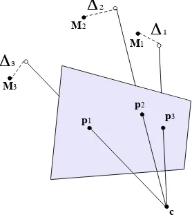
Figure 1: The orientation of the camera and the depth of the points are estimated in such a way to minimize the length of the
∆s for all the points, in a least squares sense.
To obtain the least squares solution for Eq. (3) – along the same line as in (Sch¨onemann and Carroll, 1970) – let us make explicit the residual matrix∆:
S=ZP R+1cT+ ∆. (4)
The geometric interpretation, with reference to Figure 1, is that the estimated depth defines a 3D point along the optical ray of the
image pointp, and the segment (perpendicular to the optical ray) joining this point and the corresponding reference 3D pointMis the residual. Therefore,∆is a matrix whose rows are difference vectors between reference 3D points (S) and the back-projected 2D points (P) based on their estimated depths (Z) and the esti-mated camera attitude and position (R,c).
The solution of the anisotropic OPA problem findsZ, Randcin such a way to minimize the sum of squares of the residual∆, i.e., the sum of the squared norm of the difference vectors mentioned above. This can be written as
mink∆k2
Fsubject toRTR=I (5) The problem is equivalent to the minimization of the Lagrangian function
F= tr“∆T∆”+ tr“L“RTR−I”” (6) whereLis the matrix of Lagrangian multipliers. This can be solved by setting to zero the partial derivatives ofFwith respect to the unknownsR,cand the diagonal matrixZ. The derivation of the formulae is reported in (Garro et al., 2012). It turns out that in the anisotropic case the unknowns are entangled in such a way that one must resort to the so called “block relaxation” scheme (de Leeuw, 1994), where each variable is alternatively estimated while keeping the others fixed. Algorithm 1 summarizes the pro-cedure.
Algorithm 1PROCRUSTEANEXTERIORORIENTATION Input: a set of 2D-3D correspondences(P, S)
Output: positioncand attitudeRof the camera
1. Start withZ= 0(or any guess on the depth);
5. Iterate over steps 2, 3, 4 until convergence.
In order to work toward the robust version of Algorithm 1, please note that:
• step 2 can be seen as the solution of a simple OPA problem, namely findingRsuch thatZP =R`I−1 1T/n´S; • step 3 is simply the mean along the columns of the matrix
S−ZP R.
We will return to this observation later.
3 ROBUST ESTIMATION TECHNIQUES
0 5 10 15 20 25 30 35 10−2
10−1
Iteration
Residual
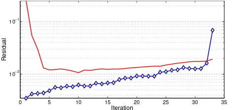
Figure 2: The(s+ 1)thresidual (diamonds) and the value of the threshold(t(1−α/2(s+1),s−k)σs)(red line) at each iteration of FS.
0 5 10 15 20 25 30 35 40 45 50
10−4 10−3 10−2 10−1 100
Point
Residual
Figure 3: Residuals at the last iteration of FS arranged in ascend-ing order. The red horizontal line is the threshold that has been exceeded.
The Least Median of Squares is a robust regression method that achieves the maximum theoretical breakdown point of0.5, i.e, it can tolerate up to 50% percent of outliers in the data without being affected. LMedS estimates the parameters of the model by minimizing the median of the absolute residuals. LetX={xi} be a set of data points and letabe ak-dimensional parameter vector to be estimated, whileri,ais the Euclidean distance be-tween a pointxi and the model determined bya. The LMedS estimate is:
ˆ
a= argmin a
median xi∈X r
2
i,a (7)
The value ofais determined using a random sampling technique. A number ofk-points subsets of thendata points is randomly selected and a parameter vectoraSis fitted to the points in each subsetS. EachaSis tested by calculating the squared residual distancer2
i,aSof each of then−kpoints inX−Sand finding the
median. TheaScorresponding to the smallest median is chosen as the estimateˆa. Ifnis the number of points in the initial set of data, there are `nk´different subsets ofkpoints that should be considered. In order to speed up the process, the number of subsets to test can be reduced to
M = log(1−p)
log(1−(1−ǫ)k, (8)
wherepis the probability of calculating the correct estimate and
ǫis the percentage of outliers.
Since LMedS is known to have a low statistical efficiency, it is important to refine the fit on a “clean” (i.e., outliers-free) set of data point. This is customarily done by computing a robust scale estimateσ∗
based on the median absolute deviation (MAD):
σ∗
= 1/φ−1(0.75)(1 + 5
n−k)
r
median xi∈X−Sˆri,
ˆ a2 (9)
whereSˆis the subset used to calculateˆa,φ−1is the inverse of the cumulative normal distribution, and1 + 5/(n−k)is a correction factor. Thenˆais refined with a least squares estimate using only the data points such that:
ri,2ˆa<(θσ
∗
)2 (10)
whereθis a constant that depends on the confidence level chosen for the test (typically around 2 or 3).
According to the taxonomy set forth in (Davies and Gather, 1993), this is a univariate single-step outlier detection procedure, that will be referred to as MAD in the following. Sequential proce-dures, on the contrary, perform successive elimination or addition of points. In particular,inward testingstarts with the whole set of data points and iteratively test the point with the highest residual
for being an outlier; it stops when the first inlier is encountered. On the contrary,outward testingstarts with an outlier-free set of points and iteratively tests the remaining points for inclusion in the clean subset, based on statistics computed on the clean subset; it stops when all the points have been processed.
Forward Search (FS) (Hadi and Simonoff, 1993, Atkinson and Riani, 2000) is an outlier detection method of the latter category. The algorithm starts from an initial subset of observations of size
m < nthat is known to be outlier free. In our case this is the setSˆfrom LMedS, andm=k. Then the iterative process starts and at everyithiteration thessamples(s=m+i−1)with the lowest residual are used to estimate the parameters of the model asand thes+ 1residualrs+1,asis monitored to detect the point
when the iteration starts including outliers.
Several monitoring heuristics have been proposed in literature. We consider here one of the simplest, that dates back to (Hadi and Simonoff, 1993); the forward search stops when:
rs2+1,as≥(t(1−α/2(s+1),s−k)σs)2 (11)
wheret(1−α/2(s+1),s−k) the1−α/2(s+ 1)quantile of the t-distribution withs−kdegrees of freedom, andσsis the standard deviation of the leastsresiduals (the residual divided byσsis also called “studentized” residual).
Figure 2 plots the(s+ 1)thresidual at each iteration: please note how the threshold adapts to the variance of the clean subset and how the residual of the first outlier pops out. Same analysis can be made on Figure 3, which plots the ordered residuals of the whole point set: the outliers are clearly separated and well above the threshold.
Theithiteration of the algorithm can be summarized as follows:
1. Estimate the parameters of the modelasusing thes=m+
i−1points in the clean subset;
2. Calculate the residualsrs+1,as of all thenpoints and
ar-range them in ascending order;
3. Test the(s+ 1)thresidual:
Ifr2s+1,as ≥(t(1−α/2(s+1),s−k)σs)2then declare all the remainingn−sobservations as outliers and stop.
Otherwise incrementi(include the(s+ 1)thpoint in the inliers).
4 ROBUST PROCRUSTEAN EXTERIOR IMAGE ORIENTATION
Resuming to the observations at the end of Section 2, one can immediately figure out that the procrustean exterior image orien-tation algorithm can be made robust against outliers by substitut-ing:
• step 2 with a robust solution (e.g., LMedS) to the problem of finding the rotation between the two point setsZP and `
I−1 1T/n´S;
• step 3 with themedianinstead of the mean along the columns ofS−ZP R.
This works pretty straightforward, and being an iterative process, convergence can be improved by re-using the estimate of the in-liers set from one iteration to the next. As customary, we used a threshold based on MAD (as described in Sec. 3) to reject outliers at each iteration.
However this simple strategy cannot recover the inlier set with high reliability foreverycondition. There are cases where FS, albeit more computationally expensive, should be used because of its superior accuracy, as experiments will show. Therefore we propose to refine the clean subset produced by the LMedS proce-dure with FS; the resulting robust procrustean exterior orientation procedure is summarized in Algorithm 2.
Algorithm 2 ROBUST PROCRUSTEAN EXTERIOR ORIENTA
-TION
Input: a set of 2D-3D correspondences(P, S)
Output: positioncand attitudeRof the camera
• Find a clean subset of three points1:
1. Start withZ= 0(or any guess on the depth);
2. ComputeRs. t. PTZ = R`I−1 1T/n´Susing LMedS (on current inliers);
3. Computec= meaninliers((S−ZP R))T;
4. ComputeZ= diag (P R(ST−c1T)) diag (P PT)−1 ;
5. Declare as inliers points that pass the test of Eq. (10);
6. Iterate over steps 2, 3, 4, 5 until convergence;
• Refine inliers estimate using FS;
• ComputeR,c, Z (algorithm (1)) considering the set of points determined in the previous step.
5 EXPERIMENTAL VALIDATION
We run synthetic experiments, usingn= {20,40,60,80,100} 3D points. The image coordinates obtained from the projection of the points have been perturbed with gaussian noise with stan-dard deviation σ = 2.0and different percentages of outliers
1Exterior orientation requires at least three points.
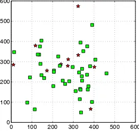
{10%,20%,30%,40%,50%}have been added to the data. Out-liers are generated by adding a random value with uniform dis-tribution in[0,100] to both coordinates of a point. The focal length of the camera was set to 500 pixel and the image size is ≈600×600(Figure 4 shows an example of synthetic image). For each value ofnand percentage of outliers the test has been run 100 times.
0 100 200 300 400 500 600 0
100 200 300 400 500 600
Figure 4: An example of the synthetic image data. The green squares are the inliers, the red stars are the outliers.
First we tested the first part of the algorithm, the one responsible for extracting a clean subset, based on LMedS, and, as expected, it provides a clean subset (with up to 50% of outliers) in most of the cases (76%). The percentage reaches 92% if one considers only a maximum of 40% of outliers. Figure 5 reports the false negative rate (see below) for the first part of the algorithm.
20 40 60 80 100 10
20 30 40 50 0 0.1 0.2 0.3 0.4
# points LMedS
% outliers
False negative rate
Figure 5: False negative rate vs percentage of outliers and number of points for the first part of the algorithm.
Then we compared empirically the robust procrustean exterior orientation method (with FS) against the baseline method with the MAD-based test only, in order to assess whether FS brings some advantage in detecting outliers.
The outlier detection stage post LMedS can be considered as a classification task, where each point has to be labelled as inlier or outlier (i.e., we test the null hypothesis that a point is an outlier)
θandαwere set to2.0and0.0001respectively, so as to yield a similar rejection threshold for a chosen reference case, corre-sponding to 100 points, 10% outliers,σ= 2.0.
20 40 60 80 100 10
20 30 40 50 0 0.5 1
# points MAD
% outliers
False negative rate
20 40 60 80 100 10
20 30 40 50 0 0.5 1
# points Forward Search
% outliers
False negative rate
20 40
60 80
100
10 20 30 40 50 0
0.5 1
% outliers MAD
# points
Accuracy
20 40
60 80
100
10 20 30 40 50 0
0.5 1
% outliers Forward Search
# points
Accuracy
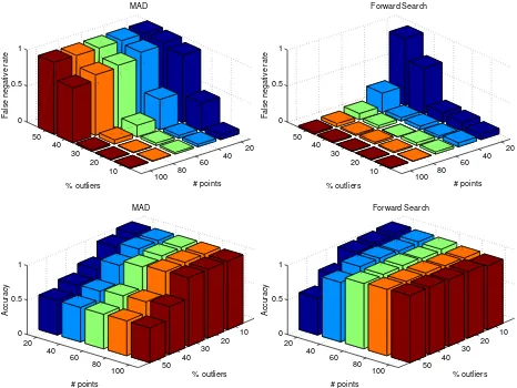
Figure 6: Top row: false negative rate vs percentage of outliers and number of points for MAD (left) and FS (right). Bottom row: accuracy vs percentage of outliers and number of points for MAD (left) and FS (right). Gaussian noise hasσ= 2.0.
oftrue positives, i.e., outliers that are correctly detected andd
be the number oftrue negatives, i.e., inliers that are correctly detected.
In order to compare the two algorithms, we monitored two figures of merit:
- thefalse negative ratedefined asc/(a+c), and
- theaccuracy, defined as(a+d)/n.
Please note that false negatives (type I error) are way more dan-gerous than false positives, as they may skew the final least squares estimate, whereas false positives (type II error) can only impact on the statistical efficiency, as they reduce the number of “good” measurements that are considered in the final least squares es-timate. For this reason, the main indicator is the false negative rate, which should be as small as possible. The accuracy indeed is monitored in order to check that the method is not achieving a low false negative rate by being too “fussy”, i.e, rejecting too many samples as outliers.
Results are reported in Fig. 6. The bar corresponding to20points and50%outliers can be considered as an extreme case and should probably left out from general considerations. The opposite case, corresponding to100points and10%outliers, is the “easy” one.
The rundown of the experiments is that with a fairly large set of point (> 60) and moderate outliers contamination (≤ 30%)
MAD and FS produce comparable results, but when the size of the data is smaller or the contamination increases, FS performs better than MAD with respect to all the indicators. This makes sense, as one could expect that the advantage of a meticulous analysis as the FS should be more noticeable on smaller samples.
Both methods are fairly unstable and produces mixed results when
n <20(results not shown here), because any statistical analysis is ineffective on such small samples.
Comparison with Fig. 5 reveals that shortfall of FS is mostly due to the first part of the algorithm failing to produce a clean subset. It also shows that FS almost never worsen the false negative rate of the clean subset and achieves high accuracy, showing that the initial clean subset has been actually extended and (almost) no outliers have been added.
6 CONCLUSIONS
REFERENCES
Ansar, A. and Daniilidis, K., 2003. Linear pose estimation from points or lines. IEEE Transactions on Pattern Analysis and Ma-chine Intelligence 25(5), pp. 578 – 589.
Atkinson, A. and Riani, M., 2000. Robust Diagnostic Regression Analysis. Springer Series in Statistics, Springer.
Beinat, A. and Crosilla, F., 2001. Generalized procrustes analy-sis for size and shape 3d object reconstruction. In: Optical 3-D Measurement Techniques, pp. 345–353.
Ben-Gal, I., 2005. Outlier detection. In: O. Maimon and L. Rokach (eds), Data Mining and Knowledge Discovery Hand-book, Springer US, New York, chapter 7, pp. 131–146–146.
Bennani Dosse, M. and TenBerge, J., 2010. Anisotropic orthogo-nal procrustes aorthogo-nalysis. Jourorthogo-nal of Classification 27(1), pp. 111– 128.
Bennani Dosse, M., Kiers, H. A. L. and Ten Berge, J., 2011. Anisotropic generalized procrustes analysis. Computational Statistics & Data Analysis 55(5), pp. 1961–1968.
Crosilla, F. and Beinat, A., 2002. Use of generalised procrustes analysis for the photogrammetric block adjustment by indepen-dent models. ISPRS Journal of Photogrammetry & Remote Sens-ing 56(3), pp. 195–209.
Davies, L. and Gather, U., 1993. The identification of multiple outliers. Journal of the American Statistical Association 88(423), pp. pp. 782–792.
de Leeuw, J., 1994. Block-relaxation algorithms in statistics. In: Information Systems and Data Analysis, Springer-Verlag, p. 308325.
Fiore, P. D., 2001. Efficient linear solution of exterior orientation. IEEE Transactions on Pattern Analysis and Machine Intelligence 23(2), pp. 140–148.
Fischler, M. A. and Bolles, R. C., 1981. Random Sample Consen-sus: a paradigm model fitting with applications to image analysis and automated cartography. Communications of the ACM 24(6), pp. 381–395.
Garro, V., Crosilla, F. and Fusiello, A., 2012. Solving the pnp problem with anisotropic orthogonal procrustes analysis. In: Sec-ond Joint 3DIM/3DPVT Conference: 3D Imaging, Modeling, Processing, Visualization and Transmission (3DIMPVT).
Gower, J., 1975. Generalized procrustes analysis. Psychometrika 40(1), pp. 33–51.
Hadi, A. S. and Simonoff, J. S., 1993. Procedures for the iden-tification of multiple outliers in linear models. Journal of the American Statistical Association 88(424), pp. pp. 1264–1272.
Haralick, R., Joo, H., Lee, C., Zhuang, X., Vaidya, V. and Kim, M., 1989. Pose estimation from corresponding point data. IEEE Transactions on Systems, Man and Cybernetics 19(6), pp. 1426 –1446.
Hesch, J. A. and Roumeliotis, S. I., 2011. A direct least-squares (dls) solution for PnP. In: Proc. of the International Conference on Computer Vision.
Horaud, R., Dornaika, F. and Lamiroy, B., 1997. Object pose: The link between weak perspective, paraperspective, and full per-spective. International Journal of Computer Vision 22, pp. 173– 189.
Kumar, R. and Hanson, A. R., 1994. Robust methods for estimat-ing pose and a sensitivity analysis. CVGIP: Image Understand-ing. 60, pp. 313–342.
Lepetit, V., Moreno-Noguer, F. and Fua, P., 2009. Epnp: An accurateo(n) solution to the pnp problem. International Journal of Computer Vision 81(2), pp. 155–166.
Lowe, D., 1991. Fitting parameterized three-dimensional models to images. IEEE Transactions on Pattern Analysis and Machine Intelligence 13(5), pp. 441 –450.
Quan, L. and Lan, Z., 1999. Linear n-point camera pose deter-mination. IEEE Transactions on Pattern Analysis and Machine Intelligence 21(8), pp. 774 –780.
Rousseeuw, P. J., 1984. Least median of squares regression. Jour-nal of the American Statistical Association 79(388), pp. pp. 871– 880.
Sch¨onemann, P., 1966. A generalized solution of the orthogonal procrustes problem. Psychometrika 31(1), pp. 1–10.
Sch¨onemann, P. and Carroll, R., 1970. Fitting one matrix to an-other under choice of a central dilation and a rigid motion. Psy-chometrika 35(2), pp. 245–255.
Stewart, C. V., 1999. Robust parameter estimation in computer vision. SIAM Review 41(3), pp. 513–537.