The Bowen ratio-energy balance method for estimating latent heat flux
of irrigated alfalfa evaluated in a semi-arid, advective environment
Richard W. Todd
∗, Steven R. Evett, Terry A. Howell
USDA-ARS, Conservation and Production Research Laboratory, P.O. Drawer 10, Bushland, TX 79012, USA
Received 15 March 2000; received in revised form 15 March 2000; accepted 17 March 2000
Abstract
The Bowen ratio-energy balance (BREB) is a micrometeorological method often used to estimate latent heat flux because of its simplicity, robustness, and cost. Estimates of latent heat flux have compared favorably with other methods in several studies, but other studies have been less certain, especially when there was sensible heat advection. We compared the latent heat flux of irrigated alfalfa (Medicago sativa, L.) estimated by the BREB method with that measured by lysimeters over a growing season in the semi-arid, advective environment of the southern High Plains. Difference statistics from the comparison and indicators of sensible heat advection were used to analyze the performance of the BREB method relative to lysimeters. Latent heat flux was calculated from mass change measured by two precision weighing lysimeters and from two BREB systems that used interchanging temperature and humidity sensors. Net radiation (Rn), soil heat flux (G), and other meteorological variables
were also measured. Difference statistics included the root mean square difference (RMSD) and relative RMSD (normalized by mean lysimeter latent heat flux). Differences between lysimeters averaged 5–15% during the day, and 25–45% at night. Estimates of latent heat flux by the two BREB systems agreed closely (relative RMSD=8%) when they were at the same location with sensors at the same height. Differences increased when the location was the same but sensors were at different heights, or when the sensor height was the same but location in the field different, and probably was related to limited fetch and the influence of different source areas beyond the field. Relative RMSD between lysimeter and BREB latent heat fluxes averaged by cutting was 25–29% during the first two cuttings and decreased to 16–19% during the last three cuttings. Relative RMSD between the methods varied from 17 to 28% during morning hours with no pattern based on cutting. Afternoon relative RMSD was 25% during the first two cuttings and decreased to 15% during subsequent cuttings. Greatest differences between the two methods were measured when the Bowen ratios were less than 0, on days that were hot, dry and windy, or when the latent heat flux exceeded the available energy (Rn−G). These conditions were likely to be encountered throughout the
growing season, but were more common earlier in the season. © 2000 Elsevier Science B.V. All rights reserved.
Keywords: Advection; Alfalfa; Bowen ratio; Energy balance; Latent heat flux; Lysimeter
Abbreviations: BREB, Bowen ratio-energy balance; PRTD, platinum resistance temperature device; DOY, day of year; RMSD, root mean square difference; IA, index of agreement
1. Introduction
The Bowen ratio-energy balance (BREB) method has been used to quantify water use (Fritschen, 1966;
∗Corresponding author. Fax:+1-806-356-5750.
E-mail address: [email protected] (R.W. Todd)
Malek et al., 1990; Wight et al., 1993; Cargnel et al., 1996), calculate crop coefficients (Malek and Bing-ham, 1993b), investigate plant–water relations (Grant and Meinzer, 1991; Malek et al., 1992; Alves et al., 1996) and evaluate crop water use models (Ortega-Farias et al., 1993; Farahani and Bausch, 1995; Todd et al., 1996). It is considered to be a fairly robust method,
and has compared favorably with other methods such as weighing lysimeters (Grant, 1975; Asktorab et al., 1989; Bausch and Bernard, 1992; Prueger et al., 1997), eddy covariance (Cellier and Olioso, 1993) or water balance (Malek and Bingham, 1993a). Most of the studies that showed agreement were conducted when Bowen ratios were mostly positive and sensible heat advection absent. Others showed less certain agree-ment (Blad and Rosenberg, 1974; Dugas et al., 1991; Xianqun, 1996).
The BREB method estimates latent heat flux from a surface using measurements of air temperature and humidity gradients, net radiation, and soil heat flux (Fritschen and Simpson, 1989). It is an indirect method, compared to methods such as eddy covari-ance, which directly measures turbulent fluxes, or weighing lysimeters, which measure the mass change of an isolated soil volume and the plants growing in it. Its advantages include straight-forward, simple measurements; it requires no information about the aerodynamic characteristics of the surface of interest; it can integrate latent heat fluxes over large areas (hundreds to thousands of square meters); it can es-timate fluxes on fine time scales (less than an hour); and it can provide continuous, unattended measure-ments. Disadvantages include sensitivity to the biases of instruments which measure gradients and energy balance terms; the possibility of discontinuous data when the Bowen ratio approaches −1, and the re-quirement, common to micrometeorological methods, of adequate fetch to ensure adherence to the assump-tions of the method.
The BREB method relies on several assumptions (Fritschen and Simpson, 1989). Transport is assumed to be one-dimensional, with no horizontal gradients. Sensors which measure gradients are assumed to be located within the equilibrium sublayer where fluxes are assumed to be constant with height. The surface is assumed to be homogeneous with respect to sources and sinks of heat, water vapor and momentum. The ratio of turbulent exchange coefficients for heat and water vapor is assumed to be 1. The first two assump-tions are usually met if adequate upwind fetch is avail-able. A fetch to height-above-surface ratio of 100:1 is often considered a rule of thumb (Rosenberg et al., 1983), although a ratio as low as 20:1 was considered adequate when Bowen ratios were small and positive (Heilman et al., 1989). Sensors at different heights
respond to different upwind source areas (Schuepp et al., 1990; Schmid, 1997), so that all sensors must have adequate fetch.
Blad and Rosenberg (1974) observed underestima-tion of latent heat flux of alfalfa by the BREB method compared to lysimeters in eastern Nebraska under sen-sible heat advection. Subsequently, Verma et al. (1978) and Motha et al. (1979) showed that the exchange co-efficient for heat was greater than that for water va-por during sensible heat advection. Lang et al. (1983) studied latent heat and sensible heat fluxes over an Australian rice paddy located in an extensive dry re-gion and found the converse when there was sensible heat advection. Based on these studies, the behavior of exchange coefficients in the presence of sensible heat advection is uncertain.
The semi-arid environment of the southern High Plains provided an opportunity to evaluate the BREB method for estimating water use of an irrigated crop under conditions of local and regional sensible heat advection. A mosaic of rangeland and dryland crops mixed with irrigated areas, and the presence of regional-scale, dry, downslope winds contribute to the advective environment experienced over much of the growing season. Our objective was to inves-tigate the performance of the BREB method in the advective environment of the southern High Plains. We compared the latent heat flux estimated by the BREB method with the latent heat flux measured by precision weighing lysimeters. Then, we used differ-ence statistics from the comparison and indicators of sensible heat advection to analyze the performance of the BREB method relative to lysimeters under a range of conditions encountered over a growing season.
2. Materials and methods
2.1. Study location
north to south and 210 m long from east to west, and was irrigated by a lateral-move sprinkler system on a schedule that met the water use demands of the crop. Dryland sorghum bordered the experimental field for 210 m to the west and a variety of dryland crops ex-tended from the south border for more than 500 m. Irrigated wheat, sorghum and corn grew for 200 m to the north, and irrigated corn, grass or soybean grew for 90–235 m along the east border of the alfalfa field, with dryland crops beyond that for more than 700 m. Alfalfa, planted in the autumn of 1995, was harvested five times in 1998 with a mean yield of 3.3 Mg ha−1 dry hay per cutting.
2.2. Weighing lysimeters
Two precision weighing lysimeters (Marek et al., 1988), 3 m×3 m×2.3 m deep were used to directly measure alfalfa evapotranspiration. They were located at the centers of the north and south halves of the experimental field. Voltages from lysimeter load cells were sampled every 6 s by a data logger (CR7, Camp-bell Scientific Inc., Logan, UT1) and 5 min averages were calculated. The evapotranspiration rate was de-termined by using the method of least squares (James et al., 1993) to find the slope of the straight line fit-ted to the six 5 min means for each half-hour period. Calibration coefficients for each lysimeter and an area correction to account for the area between the inner and outer walls of the lysimeter were applied to the slopes of each half-hour period to convert the rate of change of voltage to depth of water. We assumed that the performance of the lysimeters was consistent over the range of conditions encountered, and that they only responded to changes in mass due to water loss or gain.
2.3. The BREB method
Two identical BREB systems were used. Each con-sisted of two integrated temperature–humidity probes (THP-1, Radiation and Energy Balance Systems, Seattle, WA) inside radiation-shielded, fan-aspirated
1The mention of trade or manufacturer names is made for infor-mation only and does not imply an endorsement, recommendation, or exclusion by USDA-ARS.
housings that were mounted on a chain-driven au-tomatic exchange mechanism (AEM-1, Radiation and Energy Balance Systems, Seattle, WA). Two calibrated thin film platinum resistance tempera-ture devices (PRTDs) were incorporated in each temperature–humidity probe. One PRTD measured air temperature used to calculate the air temperature gradient and the other measured the air temperature of the humidity sensor cavity of the probe, which was used to calculate the saturation vapor pressure of wa-ter. A capacitive humidity sensor measured relative humidity. Temperature resolution of the PRTDs was 0.0056◦C, and resolution of the humidity sensor was 0.033% relative humidity. The exchange mechanism automatically switched the position of the sensors every 5 min. After each exchange, sensors were al-lowed to equilibrate with the new aerial environment for 2 min before a 3 min measurement period. Dis-tance between the sensors was 1 m. The height of sensors was periodically adjusted as alfalfa grew so that the bottom sensors were at least 1.2 times the canopy height. Maximum height of the top sensors during the study was 2 m. System 1 (SYS1) was initially installed 15 m east of the north lysimeter on DOY 111. System 2 (SYS2) was installed at the same location and sensor height on DOY 124. SYS2 subsequently remained at the north lysimeter location throughout the experiment, but the location of SYS 1 was alternated between the north and south lysime-ters. Deployment of the BREB systems is detailed in Table 1.
Table 1
Deployment of BREB systems over irrigated alfalfaa
DOY SYS1 SYS2d Mean canopy height (m)
Start End Locationb Heightc(m) Location Height (m)
111 124 N 0.5 – – 0.37
aSensor arms were 1 m apart.
bLocation indicates whether the BREB system was located near the north or the south lysimeter. cHeight indicates the height of the lower sensors.
dSYS2 was deployed on DOY 124.
2.4. Meteorological and energy balance measurements
Identically instrumented meteorological masts were centered on the north side of each weighing lysime-ter and they held a cup anemomelysime-ter (014A, Met One, Grants Pass, OR) and a temperature–humidity probe (HT225R, Rotronics, Huntington, New York) mounted 2 m above the soil surface, and a net ra-diometer (Q*5.5, Radiation and Energy Balance Systems, Seattle, WA), mounted at 1 m height that extended 1 m over the lysimeter. The radius of the source area that contributed 90% of the radiation sensed by the lower surface of the net radiometer was 1.5 m when the alfalfa was 0.5 m tall (Schmid, 1997). The radiation source area increases with shorter alfalfa and decreases with taller alfalfa. In a concurrent study, net radiation measured by a Q*5.5 net radiometer compared well with net radi-ation calculated from independent measurements of the shortwave (C14 albedometer, Kipp and Zonen, Delft, The Netherlands) and longwave (CG1/2, Kipp and Zonen, Delft, The Netherlands) components of the radiation balance (K. Copeland, personal com-munication; Rn,Q5=−6.55+1.03Rn,KZ, r2=0.99, root mean square difference (RMSD)=18.8 W m−2, mean
Rn,Q5=138.8 W m−2, mean Rn,KZ=135.9 W m−2,
n=3117). Net radiation is important to the BREB
latent heat flux estimates, and the net radiation mea-sured by similar instruments can vary considerably (Kustas et al., 1998). The absolute accuracy of net radiation was not critical to our analysis because we were interested in the relationship between BREB and lysimeter latent heat fluxes, expressed by statis-tical difference measures of the comparison, under conditions with and without evidence of sensible heat advection.
G=−30±5 W m−2. The soil water content did not vary much because of the high irrigation frequency, so that the error contributed toλEBby assuming constant soil water content was considered negligible during the day, although potentially significant at night. Soil temperature above the soil heat flux plates was mea-sured with four pairs of copper–constantan thermo-couples (304SS, Omega Engineering, Stamford, CT). Each pair had one thermocouple installed at 10 mm depth and one at 40 mm depth and they were wired in parallel to integrate the soil temperature. The same data logger that sampled the lysimeter load cells also sampled other sensors every 6 s and calculated 15 min means which were later processed as half-hour means. Net radiation and soil heat flux were averaged from measurements at the north and south lysimeter instru-ment locations to account for spatial variability be-tween the two locations.
2.5. Comparison statistics and indicators of sensible heat advection
Latent heat fluxes were compared using univari-ate, regression, and mean difference statistics given by Willmott (1982, 1984). The RMSD was calculated with
Comparison of means of half-hourly latent heat flux measured by the north (λEN) and south (λES) lysimeters
Cutting Time n MeanλEN (W m−2) MeanλES (W m−2) RMSDa (W m−2) RMSD/λEL 1-Iab
aRoot mean square difference. bIndex of disagreement.
where n is the number of half-hour observations, and
Pi and Oi are half-hour observations of the two vari-ables being compared. The RMSD is a conservative absolute difference measurement because it is more sensitive to extreme differences (Willmott, 1984) and can be considered a high estimate of the actual average difference (Willmott, 1982). The RMSD expressed as a percentage of either the mean of the two lysimeters,
λEL, or the mean of the two BREB systems,λEB, was used as a measure of relative difference. The index of agreement (IA) is a relative difference measure calcu-lated with
whereO¯ is the mean of variable O (Willmott, 1982). Perfect agreement between P and O would be ex-pressed by IA=1.
We used the definition of Rosenberg et al. (1983), where advection is the “transport of energy or mass in the horizontal plane in the downwind direction.” Sen-sible heat advection was not directly measured, but was inferred when the ratio of mean lysimeter latent heat flux to available energy (Rn−G) was greater than
resistance ra. Thom (1975) pointed out that this ra-tio will be very large if there is a strong, dry air flow over vegetation, which he called an ‘oasis situation’. The ratio was calculated from meteorological mea-surements at the north lysimeter using expressions given by Thom (1975) for the climatological resis-tance and the aerodynamic resisresis-tance uncorrected for thermal stability:
ri
ra
= ρacpD[γ (Rn−G)] −1 [ln((z−d)/z0)]2(k2u)−1
(3)
where the saturation vapor pressure deficit D (kPa), was calculated from the temperature and humidity measured at z=2 m, d is the zero plane displacement height (m), estimated as 0.63zc (zc is the canopy height), z0, estimated as 0.13zc, is the roughness length (m), k=0.41 is von Karmen’s constant, and
u is the wind speed at a height of 2 m (m s−1). The ratio becomes very large when aerial conditions are warm, dry, and windy, as were encountered on days with evidence of sensible heat advection.
3. Results and discussion
3.1. Weighing lysimeter variability
Factors that contribute to the variability between lysimeter measurements include environmental dif-ferences due to field position or difdif-ferences in crop density, development or leaf area. We examined the variability about the mean of the latent heat flux measurements of the two weighing lysimeters by calculating the RMSD where λEN,i andλES,i were half-hour observations of latent heat flux at the north and south lysimeters, respectively. Relative difference was calculated by normalizing the RMSD by the mean latent heat flux of the two lysimeters. During the daytime (0700–1900 h), mean relative RMSD by cutting ranged from 7 to 17% (Table 2). At night (1900–0700 h), relative RMSD ranged from 29 to 59% (Table 2). Variability was greater at night be-cause 52% of the night-time half-hour observations were less than the 0.05 mm h−1 resolution of the lysimeters. Index of disagreement (1-IA) was less, ranging from 2 to 14% during the daytime and from 10 to 44% at night. Based on this analysis, a
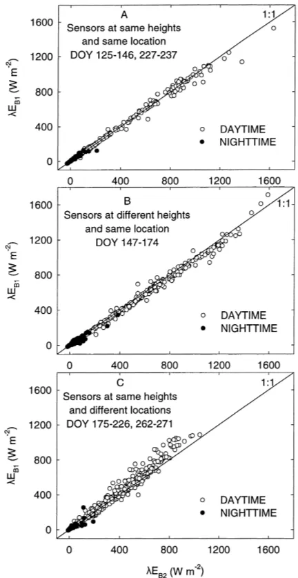
reason-Fig. 1. Comparisons of latent heat flux estimated by two BREB systems, with three deployments. SYS1 (λEB1) was near the north lysimeter (A, B) or near the south lysimeter (C). SYS2 (λEB2) was always near the north lysimeter. Other details are given in Table 1.
3.2. Comparison of BREB systems
The tests of Ohmura (1982) indicated counter-gradient fluxes usually during the early morning hours. Bowen ratios near −1 were most likely be-tween 1730 and 1930 h on days when the sensible heat flux towards the canopy was a significant component of the energy balance. Retention of data ranged from 85 to 94% of the daytime half-hour observations of the five cuttings. Over the season, 91% of daytime ob-servations were valid. At night, 71% of the half-hour observations were valid. The BREB estimates of la-tent heat flux behaved erratically on the days when alfalfa was irrigated. As the temperature and humid-ity measured by the BREB sensors were integrated over a large area of the alfalfa field, they were often affected by irrigation even after the irrigation system passed over the sensors. The magnitude of this effect depended on wind direction. Also, when the irriga-tion system passed over the BREB systems, drop nozzles wetted the lower sensor arm, while the upper sensor arm remained dry. Lysimeter measurements during irrigation or precipitation, recorded as mass gains, were also uncertain. Therefore, days with irri-gation or significant precipitation were excluded from analysis.
The two BREB systems, with sensor pairs at the same heights and positioned near the north lysime-ter, had similar estimates of latent heat flux (Fig. 1A). Daytime RMSD between the two systems was 8% of the mean latent heat flux of the two systems, and 1-IA was 1% (Table 3). Relative difference measures between lysimeters during this deployment were 16 and 6% for the normalized RMSD and 1-IA, respec-tively. Less variability between the BREB systems
Table 3
Comparison of means of half-hourly latent heat flux estimated by BREB SYS1 (λEB1) and SYS2 (λEB2)
Deploy Time n MeanλEB1 (W m−2) MeanλEB2 (W m−2) RMSDa RMSD/λEB 1-Iab
Same Day 210 426 427 33 0.08 0.01
Night 179 18 19 9 0.49 0.07
Different height Day 311 588 608 38 0.06 0.02
Night 172 37 39 15 0.39 0.10
Different location Day 411 443 417 57 0.13 0.07
Night 316 11 9 12 1.20 0.32
aRoot mean square difference. bIndex of disagreement.
compared to that between lysimeters was probably be-cause the BREB systems spatially integrated the same area, while the lysimeter measurements each repre-sented a discrete 9 m2area. During night-time hours, the two BREB systems also agreed closely, although the relative difference between them increased com-pared to the daytime case (Table 3).
When the systems were located near the north lysimeter but at different heights (SYS1 sensors were 0.25 or 0.5 m higher, Table 1),λEB2 was consistently greater thanλEB1(Fig. 1B). Relative difference of the latent heat flux between the two systems was slightly different compared to when the systems were at the same height, with a relative RMSD of 6% and a 1-IA of 2% (Table 3). Most of the time, with the sensors of the two systems separated by up to 0.5 m, latent heat flux decreased with height. Two factors, both related to fetch, may explain this. First, sensors at different heights experienced different upwind source footprints. For example, cumulative relative flux, the fraction of flux that originated from the alfalfa field (Schuepp et al., 1990), was always less for the higher sensors of SYS1. Mean cumulative relative flux for the top sensor of SYS1 during this deployment was 0.78, compared to mean cumulative relative flux for the top sensor of SYS2 of 0.83. Higher sensors were more affected by areas beyond the alfalfa field. Sec-ond, under the commonly encountered conditions of warmer, drier air moving horizontally over the cooler, moister air above the alfalfa field, and high wind speeds, latent heat may have been diverted from the vertical flow into the horizontal flow, so the assump-tion that flux was constant with height was invalid.
Table 4
A comparison of two days which showed disagreement (DOY 219) or agreement (DOY 224) between the BREB systems deployed at the same heights and located near the south lysimeter (SYS1) or the north lysimeter (SYS2)a
DOY Wind direction λEL/(Rn−G) South lysimeter North lysimeter
Air temperature, D u λEB1 Air temperature, D u λEB2 T (◦C) (kPa) (m s−1) (W m−2) T (◦C) (kPa) (m s−1) (W m−2)
219 S to SW 1.32 27.6 2.08 4.6 553 27.0 1.91 4.1 492
224 W to NW 1.02 24.8 0.99 2.7 357 25.0 1.14 2.7 361
aAir temperature, saturation vapor pressure deficit (D) and wind speed (u) were measured at 2 m above each lysimeter. All means are for the daytime (0700–1900 h).
lysimeter and the other at the south lysimeter, sepa-rated by 225 m (Table 1). For this deployment,λEB1, located near the south lysimeter, was usually greater thanλEB2, located near the north lysimeter (Fig. 1C). Variability between the two systems increased com-pared to the previously discussed deployments. Nor-malized RMSD was 13% and 1-IA was 7% (Table 3). Part of the greater variability observed between the two BREB systems during this deployment was be-cause the systems usually had different fetch and expe-rienced different upwind footprints. Two days which illustrate this are contrasted in Table 4 and Fig. 2. On DOY 219, winds were predominantly from the south to southwest andλELexceeded Rn−G by 32%. On DOY 224, winds blew from the west to northwest and there was little evidence of sensible heat advection. Air tem-perature, vapor pressure deficit and wind speed were greater on DOY 219, andλEB1(near the south lysime-ter) was greater thanλEB2 (near the north lysimeter) throughout the daytime hours (Fig. 2A), while on DOY 224,λEB1andλEB2agreed very closely (Fig. 2B).
3.3. Comparison of lysimeter and BREB latent heat fluxes
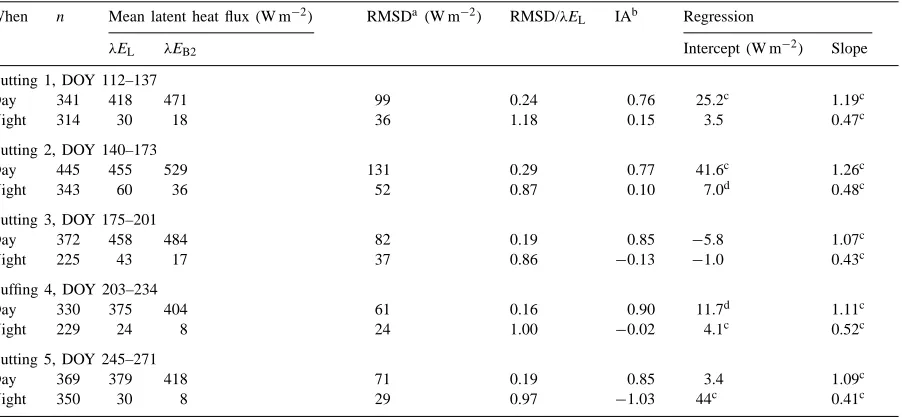
We assumed that lysimeters only responded to change in mass from water loss or gain, so that they provided a baseline latent heat flux that responded consistently over a wide range of conditions. Latent heat flux estimated by SYS2 (λEB2) located near the north lysimeter was compared with the mean latent heat flux measured by the two lysimeters, because it usually experienced the greatest fetch. Disagreement between the BREB and lysimeter daytime latent heat fluxes was greatest during the first and the second
cutting, when the relative RMSD was 24 and 29%, respectively (Table 5). Daytime relative RMSD de-creased during subsequent cuttings, and ranged from
Table 5
Univariate, regression and mean difference comparisons of half-hour measurements of mean latent heat flux (λEL) and latent heat flux estimated by the BREB system located near the north lysimeter (λEB2)
When n Mean latent heat flux (W m−2) RMSDa (W m−2) RMSD/λEL IAb Regression
λEL λEB2 Intercept (W m−2) Slope
Cutting 1, DOY 112–137
Day 341 418 471 99 0.24 0.76 25.2c 1.19c
Night 314 30 18 36 1.18 0.15 3.5 0.47c
Cutting 2, DOY 140–173
Day 445 455 529 131 0.29 0.77 41.6c 1.26c
Night 343 60 36 52 0.87 0.10 7.0d 0.48c
Cutting 3, DOY 175–201
Day 372 458 484 82 0.19 0.85 −5.8 1.07c
Night 225 43 17 37 0.86 −0.13 −1.0 0.43c
Cuffing 4, DOY 203–234
Day 330 375 404 61 0.16 0.90 11.7d 1.11c
Night 229 24 8 24 1.00 −0.02 4.1c 0.52c
Cutting 5, DOY 245–271
Day 369 379 418 71 0.19 0.85 3.4 1.09c
Night 350 30 8 29 0.97 −1.03 44c 0.41c
aRoot mean square difference. bIndex of agreement.
cIntercept was significantly different from 0 or slope was significantly different from 1 at the p<0.01 level. dIntercept was significantly different from 0 or slope was significantly different from 1 at the p<0.05 level.
16 to 19%. IA and regression statistics also indicated greater disagreement between the two methods during the first two cuttings compared to the later cuttings (Table 5). Greatest disagreement was when the la-tent heat flux densities were greater than 400 W m−2 (Fig. 3). Night-time latent heat flux of the two
meth-Table 6
Mean latent heat flux estimated by the BREB system located near the north lysimeter (λEB2) and measured by lysimeters, and the difference measures of BREB estimates compared with lysimeter-measured latent heat flux, by morning and afternoon within cutting
Cutting Morninga Afternoonb
n λEL λEB2 RMSDc RMSD/ IAd n λEL λEB2 RMSD ) RMSD/ IA
(W m−2) (W m−2) (W m−2) λEL (W m−2) (W m−2) (W m−2) λEL
1 159 419 470 85 0.20 0.78 147 476 535 115 0.24 0.63
2 191 436 517 122 0.28 0.77 198 546 623 145 0.26 0.71
3 164 463 506 78 0.17 0.85 162 519 529 89 0.17 0.78
4 145 386 429 66 0.17 0.87 148 418 441 57 0.14 0.90
5 173 368 434 79 0.21 0.79 162 453 478 64 0.14 0.83
aMorning hours were from 0800 to 1300 h. bAfternoon hours were from 1300 to 1800 h. cRoot mean square difference.
dIndex of agreement.
ods disagreed more than the daytime fluxes. Relative RMSD, by cutting, ranged from 86 to 118%, and no pattern related to cutting was detected (Table 5).
Fig. 3. Comparisons of half-hour latent heat flux estimated by the BREB method (λEB2) with mean half-hour latent heat flux measured by lysimeters (λEL), by alfalfa cutting. Open circles are daytime measurements (0700–1900 h) and closed circles are night-time measurements.
exceededλELduring the daytime hours. The only ex-ceptions were during late afternoon when there were few BREB measurements in a half-hour mean because of invalid data. During subsequent cuttings,λEB2was greater thanλELduring the daytime morning and early afternoon hours, but agreed more closely later in the afternoon. Mean half-hourλEB2was consistently less thanλEL during the night-time hours. Disagreement of the BREB method with lysimeters appeared to have two components. There was a consistent disagreement during the morning hours which was common from
Fig. 4. Mean diel latent heat flux measured by lysimeters (λEL) and estimated by the BREB method (λEB2), by cutting.
3.4. The Bowen ratio versus relative difference between BREB and lysimeter latent heat fluxes
Half-hour daytime λEB2 andλEL were compared for each day and the RMSD of each day normalized by mean daytime λEL. We then calculated a mean daytime Bowen ratio with βEB=HR/λEL, where Rn,
G and λEL were measured and sensible heat flux,
HR, was the residual term of the energy balance. The BREB method estimated the latent heat flux best when βEBwas between 0 and 0.3 (Fig. 5). Relative
RMSD was within the relative RMSD observed be-tween lysimeters during the daytime on 17 out of 86 days. The relative difference increased both as
Fig. 5. Relative root mean square difference (RMSD/λEL) of the daytime BREB and lysimeter latent heat flux comparison correlated with the energy balance Bowen ratio, by days within leaf area index (LAI) class.
3.5. Indicators of sensible heat advection versus relative difference between BREB and lysimeter latent heat fluxes
Relative RMSD of daytime latent heat flux in-creased linearly as ri/ra increased and was evident for all cuttings (Fig. 6). Days during the first two cut-tings showed the greatest relative difference and the greatest ri/ra. Greatest difference between lysimeter measurements and the BREB estimate of latent heat
Fig. 6. Relative root mean square difference (RMSD/λEL) of the daytime BREB and lysimeter latent heat flux comparison correlated with the ratio of climatological resistance (ri) to aerodynamic
resistance (ra), by days within cutting.
Fig. 7. Relative root mean square difference (RMSD/λEL) of the daytime BREB and lysimeter latent heat flux comparison correlated with the ratio of latent heat flux to available energy, by days within cutting.
flux occurred on days that were hot, dry, and windy. The mean daytime BREB and lysimeter latent heat fluxes agreed most closely when the ratio of latent heat flux to available energy (Rn−G) was around 1.0 (Fig. 7). Relative RMSD increased to values greater than 0.3 as the ratio increased to more than 1.5.
4. Summary and conclusions
Variability about the mean latent heat flux measured by the two precision weighing lysimeters during the daytime was generally within 5–15%. Night-time vari-ability was greater, on the order of 25–45%. On an average, 91% of half-hour daytime observations and 71% of night-time observations of latent heat flux by the BREB method were valid. Estimates of latent heat flux by the two BREB systems agreed closely when they were at the same location with sensors at the same height. Differences increased when the location was the same but the sensors were at different heights, or when the sensor height was the same but location in the field different, and probably was related to lim-ited fetch and the influence of different source areas beyond the field.
three cuttings. Relative RMSD between the methods varied during morning hours with no pattern based on cutting. Afternoon relative RMSD was 25% during the first two cuttings and decreased to 15% during subsequent cuttings. Greatest differences between the two methods were measured when the Bowen ratios were less than 0, on days that were hot, dry and windy, or when the latent heat flux exceeded the available energy (Rn−G). These conditions were likely to be
encountered throughout the growing season, but were more common during the first two cuttings.
Acknowledgements
This research was partly funded by the USAID Agricultural Technology Utilization and Transfer Project. The authors express their appreciation to Karen Copeland, soil scientist, and Don Dusek, agronomist, for lysimeter maintenance, and collec-tion and processing of lysimeter data; and to bio-logical technicians Brice Ruthardt and Jim Cresap, who maintained and irrigated the research field and collected plant data.
References
Alves, I., Perrier, A., Pereira, L.S., 1996. Penman–Monteith equation: how good is the ‘big leaf ? In: Camp, C.R., Sadler, E.J., Yoder, R.E. (Eds.), Evapotranspiration and Irrigation Scheduling, Proceedings of the International Conference, San Antonio, TX, 3–6 November, 1996. Am. Soc. Agric. Eng., St. Joseph, MI, pp. 599–605.
Asktorab, H., Pruitt, W.O., Paw, U.K.T., George, W.V., 1989. Energy balance determinations close to the soil surface using a micro Bowen ratio system. Agric. For. Meteorol. 46, 259–274. Bausch, W.C., Bernard, T.M., 1992. Spatial averaging Bowen ratio system: description and lysimeter comparison. Trans. ASAE 35, 121–129.
Blad, B.L., Rosenberg, N.J., 1974. Lysimetric calibration of the Bowen ratio-energy balance method for evapotranspiration estimation in the central Great Plains. J. Appl. Meteorol. 13, 227–236.
Cargnel, M.D., Orchansky, A.L., Brevedan, R.E., Luayza, G., Palomo, R., 1996. Evaptranspiration measurements over a soybean crop. In: Camp, C.R., Sadler, E.J., Yoder, R.E. (Eds.), Evapotranspiration and Irrigation Scheduling, Proceedings of the International Conference, San Antonio, TX, 3–6 November 1996. Am. Soc. Agric. Eng., St. Joseph, MI, pp. 304–308. Cellier, P., Olioso, A., 1993. A simple system for automated
longterm Bowen ratio measurement. Agric. For. Meteorol. 66, 81–92.
Dugas, W.A., Fritschen, L.J., Gay, L.W., Held, A.A., Matthias, A.D., Reicosky, D.C., Steduto, P., Steiner, J.L., 1991. Bowen ratio, eddy correlation, and portable chamber measurements of sensible and latent heat flux over irrigated spring wheat. Agric. For. Meteorol. 56, 1–20.
Farahani, H.J., Bausch, W.C., 1995. Performance of evapotranspiration models for maize — bare soil to closed canopy. Trans. ASAE 38, 1049–1059.
Fritschen, L.J., 1966. Evapotranspiration rates of field crops determined by the Bowen ratio method. Agron. J. 58, 339–342. Fritschen, L.J., Simpson, J.R., 1989. Surface energy balance and radiation systems: general description and improvements. J. Appl. Meteorol. 28, 680–689.
Grant, D.R., 1975. Comparison of evaporation measurements using different methods. Q.J.R. Met. Soc. 101, 543–550.
Grant, D.A., Meinzer, F.C., 1991. Regulation of transpiration in field-grown sugarcane: evaluation of the stomatal response to humidity with the Bowen ratio technique. Agric. For. Meteorol. 53, 169–183.
Heilman, J.L., Brittin, C.L., Neale, C.M.U., 1989. Fetch requirements for Bowen ratio measurements of latent and sensible heat fluxes. Agric. For. Meteorol. 44, 261–273. James, M.L., Smith, G.M., Wolford, J.C., 1993. Applied Numerical
Methods for Digital Computation, 4th Edition. Harper Collins College Publishers, New York.
Kustas, W.P., Prueger, J.H., Hipps, L.E., Hatfield, J.L., Meek, D., 1998. Inconsistencies in net radiation estimates from use of several models of instruments in a desert environment. Agric. For. Meteorol. 90, 257–263.
Lang, A.R.G., McNaughton, K.G., Fazu, C., Bradley, E.F., Ohtaki, E., 1983. Inequality of eddy transfer coefficients for vertical transport of sensible and latent heats during advective inversions. Boundary-Layer Meteorol. 25, 25–41.
Malek, E., Bingham, G.E., 1993a. Comparison of the Bowen ratio-energy balance and the water balance methods for the measurement of evapotranspiration. J. Hydrol. 146, 209–220. Malek, E., Bingham, G.E., 1993b. Growing season
evapotranspi-ration and crop coefficient. In: Allen, R.G., Van Bavel, C.M.U. (Eds.), Management of Irrigation and Drainage Systems, Integrated Perspectives. Am. Soc. Civ. Eng., New York, pp. 961–968.
Malek, E., Bingham, G.E., McCurdy, G.D., 1990. Evapo-transpiration from the margin and moist playa of a closed desert valley. J. Hydrol. 120, 15–34.
Malek, E., Bingham, G.E., McCurdy, G.D., 1992. Continuous measurement of aerodynamic and alfalfa canopy resistances using the Bowen ratio-energy balance and Penman–Monteith methods. Boundary-Layer Meteorol. 59, 187–194.
Marek, T.H., Schneider, A.D., Howell, T.A., Ebeling, L.L., 1988. Design and installation of large weighing monolithic lysimeters. Trans. ASAE 31, 477–484.
Motha, R.P., Verma, S.B., Rosenberg, N.J., 1979. Exchange coefficients under sensible heat advection determined by eddy correlation. Agric. Meteorol. 20, 273–280.
Ohmura, A., 1982. Objective criteria for rejecting data for Bowen ratio flux calculations. J. Appl. Meteorol. 21, 595–598. Ortega-Farias, S.O., Cuenca, R.H., English, M., 1993. Hourly
methods. In: Allen, R.G., Van Bavel, C.M.U. (Eds.), Management of Irrigation and Drainage Systems, Integrated Perspectives. Am. Soc. Civil Eng., New York, pp. 969–976. Prueger, J.H., Hatfield, J.L., Aase, J.K., Pikul Jr., J.L., 1997.
Bowen-ratio comparisons with lysimetric evapotranspiration. Agron. J. 89, 730–736.
Rosenberg, N.J., Blad, B.L., Verma, S.B., 1983. Microclimate: the Biological Environment. Wiley, New York, 495 pp.
Schmid, H.P., 1997. Experimental design for flux measurements: matching scales of observations and fluxes. Agric. For. Meteorol. 87, 179–200.
Schuepp, P.H., Leclerc, M.Y., MacPherson, J.I., Desjardins, R.L., 1990. Footprint prediction of scalar fluxes form analytical solutions of the diffusion equation. Boundary-Layer Meteorol. 50, 355–373.
Thom, A.S., 1975. Momentum, mass, and heat exchange. In: Monteith, J.L. (Ed.), Vegetation and the Atmosphere, Vol. 1. Academic Press, New York, pp. 57–109.
Todd, R.W., Klocke, N.L., Arkebauer, T.J., 1996. Latent heat fluxes from a developing canopy partitioned by energy balance-combination models. In: Camp, C.R., Sadler, E.J., Yoder, R.E. (Eds.), Evapotranspiration and Irrigation
Scheduling, Proceedings of the International Conference, San Antonio, TX, 3–6 November 1996. Am. Soc. Agric. Eng., St. Joseph, MI, pp. 606–612.
Verma, S.B., Rosenberg, N.J., Blad, B.L., 1978. Turbulent exchange coefficients for sensible heat and water vapor under advective conditions. J. Appl. Meteorol. 17, 330–338. Wight, J.R., Hanson, C.L., Wright, J.L., 1993. Comparing Bowen
ratio-energy balance systems for measuring ET. In: Allen, R.G., Van Bavel, C.M.U. (Eds.), Management of Irrigation and Drainage Systems, Integrated Perspectives. Am. Soc. Civ. Eng., New York, pp. 953–960.
Willmott, C.J., 1982. Some comments on the evaluation of model performance. Bull. Am. Meteorol. Soc. 63, 1309–1313. Willmott, C.J., 1984. On the evaluation of model performance