IPGS - UMR 7516 CNRS, University of Strasbourg, Strasbourg, France
Commission II, WG II/6
KEY WORDS:interactive visualization, modern GPU techniques, geological displacements
ABSTRACT:
Quantifying and visualizing deformation and material fluxes is an indispensable tool for many geoscientific applications at different scales comprising for example global convective models (Burstedde et al., 2013), co-seismic slip (Leprince et al., 2007) or local slope deformation (Stumpf et al., 2014b). Within the European project IQmulus (http://www.iqmulus.eu) a special focus is laid on the efficient detection and visualization of submarine sand dune displacements. In this paper we present our approaches on the visualization of the calculated displacements utilizing modern GPU techniques to enable the user to interactively analyze intermediate and final results within the whole workflow.
1. INTRODUCTION
Advances in stereo-photogrammetry, laser scanning and multi-beam echo sounding (MBES) continuously increase the availabil-ity of multi-temporal measurements of the land- and sub-marine topography opening new possibilities to study the dynamics of geomorphological and geological processes. In particular sub-marine dunes and sand banks are among the most dynamic geo-morphological formations in coastal waters. They play an impor-tant role in the sediment transfer and their movement can have significant impacts on the benthic ecosystem, marine transport in coastal waters, and infrastructure such as pipelines and commu-nication cables. While in the past it has been difficult to observe the dune dynamics directly recent advances in MBES now en-able increasingly frequent observations of the sea floor morphol-ogy. Currently, the prevailing standard for the analysis of multi-temporal MBES surveys is, however, visual analysis by trained experts delineating the crest line of the dunes at several time steps using commercial or open-source GIS software (Xu et al., 2008, Van Landeghem et al., 2012).
A few studies have demonstrated the feasibility of using image correlation techniques for measuring dune migration (Franzetti et al., 2013, Duffy and Hughes-Clarke, 2005) but to the best of our knowledge integrated workflows that enable the derivation and interactive visualization of sub-marine dune migration are not yet available. To fill this gap a new workflow for the automatic detec-tion of marine sand dune displacements was implemented within the IQmulus project utilizing a cloud infrastructure to process the large input data and GPU technology for efficient interactive vi-sualization.
2. DISPLACEMENT MEASUREMENT WORKFLOW
Measuring vertical deformation from multi-temporal point cloud datasets is generally a straight forward operation for globally flat
∗Corresponding author
surfaces, whereas the derivation of 2D displacement comprises greater ambiguity and requires a robust matching technique.
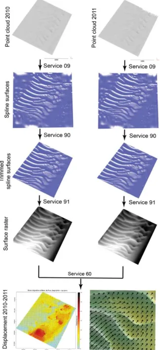
The overall implemented workflow is presented in Figure 1 and includes several processing steps that are available as services in the cloud IQmulus cloud infrastructure.
Preceding the bi-temporal matching Locally Refined B-Splines (Skytt et al., 2015, Dokken et al., 2013) are used to approximate the point cloud with a continuous surface representation (Service 09). Since the LR B-Splines also extrapolates a surface beyond the extent of the input point clouds the surface is trimmed in a subsequent step to the spatial extent of the input (Service 90). The generated surface is than sampled at regular intervals (the target resolution can be defined by the user) to produce a regularly gridded digital elevation model (DEM, Service 91).
In the final step both grids are analyzed jointly using an image correlation technique (Service 60) which is based on the open-source library MicMac (Deseilligny et al., 2015). The technique has been developed with a focus on optical image correlation (Rosu et al., 2015) and was demonstrated to provide be more ro-bust and faster matching results than comparable tools for mea-suring dune migration from multi-temporal DEMs (Stumpf et al., 2014a).The underlying algorithm implements a coarse-to-fine hi-erarchical correlation scheme where a template patch from one DEM is matched within a certain search range to all possible posi-tions in the second DEM. The matching cost among the patches is evaluated using the normalized cross-correlation coefficient and an extra regularization term which imposes a constraint on the smoothness of the derived displacement field. Sub-pixel preci-sion is achieved by oversampling of the input data. The algo-rithm is parallelized and can therefore exploit all available cores of a single virtual machine within the IQmulus cloud. During the workflow the outputs of the LR B-Spline interpolation can be vi-sualized interactively to optimize free algorithm parameters for the particular application.
partic-Figure 2: Details illustrating the LR B-Spline rendering technique. The surface consists of a set of elements, outlined in black (left). These elements are rendered using tessellated patches outlined in green (center). The number of triangles used to render each patch varies depending on the screen size of the elements within that patch. The right figure shows an exaggeration of the interactive level of detail, constructed by setting an artificially high error tolerance when computing the number of triangles per patch. Notice that the resulting triangle mesh is water tight. The dataset shown is from the Barringer Crater, Arizona.
Figure 1: Marine Sand Dunes displacement: Complete workflow from original point clouds (top) over LR-spline surfaces (middle) to final result visualization (bottom)
ular hierarchical level has finished and while the the computation continues on the next finer level. The complete workflow is im-plemented as a series of modular services which can be called in isolation or as a sequence sharing the same HDFS storage and cloud infrastructure. All illustrations are based on processing re-sults derived from two MBES surveys of the Banc de Four dune field (offshore Western Britanny, France) covering approximately 10km2
.
3. VISUALIZATION
To interactively analyze the intermediate and final results of the workflow we use visualization techniques utilize modern GPU based methods to achieve interactive rates which are described in the next sections.
3.1 Smooth surface representations
Most real-world terrains can be represented as smooth surfaces at a given scale, and this is today utilized by many regular storage formats such as Digital Elevation Models (DEMs). DEMs are raster-based and represent the altitude at a certain spatial location as an elevation above a datum. Unfortunately, reconstructing the real terrain from this DEM is non-trivial and requires knowledge from its construction: should the DEM be interpreted as a col-lection of point values, a colcol-lection of piecewise planar cell aver-ages, a bilinear surface, a bicubic surface, or something along the lines of a regular triangular mesh (and if so: how to choose the diagonals that splint each quadrilateral into two triangles)? Even after this reconstruction we know that the model of the terrain, and the terrain itself will differ, especially where the terrain has large changes in altitude in neighboring DEM cells.
A major drawback of DEMs is that they are very poor at adapt-ing to changes in smoothness over the terrain: a flat salt lake will require just as many points to represent as a rocky hillside. An alternative is to use triangulated irregular networks in which the size of each triangle will vary over the terrain: Where there are abrupt changes the triangles can be made small to capture the high frequencies in the terrain, and similarly the triangles can be made larger where the terrain is smooth. However, the terrain is still represented as a piecewise planar surface. An improvement on this is to use a higher-order representation of the terrain. In engineering and computer aided design non-uniform rational B-splines (NURBS) are predominant to represent higher-order sur-faces. NURBS surfaces are excellent at representing high-order surfaces with a limited extent, but unfortunately do not adapt very well to local changes in smoothness as the whole surface is a ten-sor product of two NURBS curves.
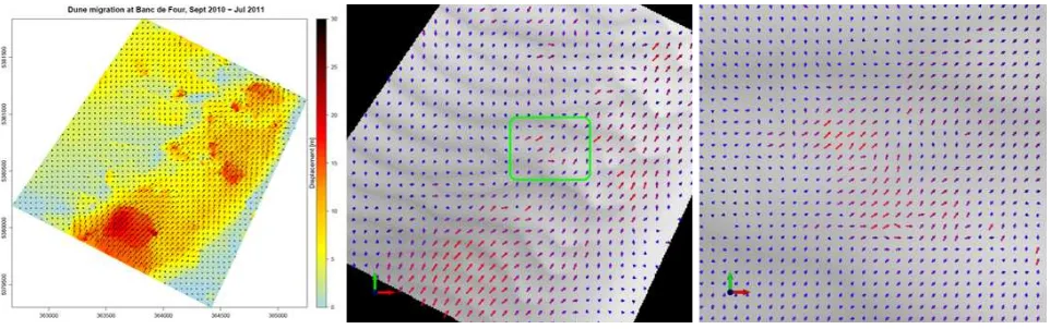
Figure 3: LR-Spline surface (left), combined with full input point cloud (middle) and showing only input points with high error compared to the reconstructed surface (right). The thresholding of points according to their distance to the surface is interactive, and enables a user to quickly inspect the quality of the spline surface.
Figure 4: Interactive dynamic glyphs: Usual static result image (left), using interactive glyphs (middle), zoomed in view using glyphs (right)
3.2 Creating and rendering LR B-splines
An MBES survey can result in a point cloud with millions of points for a limited area, and constructing an LR B-spline directly is therefore a computationally demanding task. The LR B-Spline adapts to the features of the terrain, with more elements close to sharp features, and similarly fewer elements in smooth areas.
The rendering and visualization of raster and triangulated irregu-lar networks has been well studied in the literature before. Ren-dering of NURBS surfaces is also well established. However, rendering of LR B-Splines has only recently been accomplished (Hjelmervik and Fuchs, 2015).
GPUs support only polygonal meshes, and we therefore need to convert the LR spline representation to a triangulation, referred to as a tessellation. A classical approach is here to perform a uni-form sampling of the surface in either the geometry or parameter space, yet this will often either produce too many or too few tri-angles. Too many triangles will severely impact the interactivity when navigating a scene, whilst too few triangles will dramati-cally reduce the quality of the visualization. The optimal num-ber of triangles will furthermore vary as the camera navigates the scene since an element close to the camera will cover more screen area than an equally large element further away.
Hjelmervik et al. (Hjelmervik and Fuchs, 2015) demonstrated how one can construct a pixel perfect visualization of an LR B-spline based on these observations and through using the hard-ware tessellator found in modern GPUs. First, the Bezier coef-ficients of the LR B-Spline are extracted together with an accel-eration datastructure. A set of patches are then rendered using
OpenGL to cover the full extent of the surface. Each patch con-sists of a set of elements in the LR B-Spline surface, and is tessel-lated according to a view dependent criteria that guarantees that each triangle covers at most one single pixel. Unfortunately, this is not sufficient to guarantee a pixel perfect rendering as cracks will often appear on the border between two neighboring patches when they do not agree on the tessellation level across the edge. This can be addressed by forcing neighboring patches to use the same tessellation level on the shared edge.
The tessellation is performed in its entirety on the GPU itself for every single frame that is rendered. The patches are simi-larly converted on-the-fly by the hardware tessellator to triangles, yielding an interactive view-dependent level of detail with a per-pixel-accurate rendering. On modern GPUs, this approach yields highly interactive framerates (Hjelmervik and Fuchs, 2015).
not only generate the glyph, but also take the size of the glyph in screen space into account to choose an appropriate level of tessellation (view dependent tessellation). The bigger the glyph would be on the screen the more it is tessellated, which allows for a smooth visual display. In contrast to a static image, the vi-sualization is interactive and can be zoomed to different points of interest. The glyphs are automatically recalculated according to the users viewpoint, e.g. size, number/density of glyphs, and tessellation level (see Figure 4).
(a) Glyph length
(b) Data array
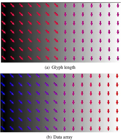
Figure 5: Color mapping glyph length (a) and color mapping data array (b)
3.3.1 Glyph Properties The user interface of the visualiza-tion system exposes the main properties of the glyph genera-tion for interactive selecgenera-tion and adjustment. These properties include:
Glyph spacing: The spacing property controls how the glyphs are distributed on screen. The distribution is affected by two values: Spacing Mode and the Goal Spacing. The Goal Spacing defines a target value for the number of screen pixels separating the cen-ter of two glyphs. If the Spacing Mode is set to Default, this is the actual distance between the glyphs. Two additional spacing modes are available, namely Power of 2, which creates the next power of two number of glyphs that results in a spacing close to the goal spacing, and Whole Fraction, which performs an analo-gous spacifing based on arbitrary integers.
Arrow properties: These settings control the appearance of the glyph. The LOD factor controls the GPU-based tessellation of the arrow glyphs. It is a target value for the maximum number of
a scalar value for color mapping. The source of this value is either the length of the aforementioned vector(x, y)T
, which also de-termines its length and direction, or a sample from an additional data array. The result of the two different modes can be seen in Figure 5.
3.3.2 Glyph Tessellation Details Depending on their on-screen size and the current LOD factor value the glyphs are tessellated with a different amount of detail. Each glyph starts out as two cubes where the overlapping faces are removed. One of the cubes will be tapered to form the arrow’s head, the other one will be scaled along one axis to form the arrow’s tail. They are tessel-lated, projected to a cylindrical shape and rendered to create the arrow glyphs. The result for different tessellation resolutions are shown in Figure 6.
Figure 6: Glyph tessellation resolution: low (left), middle (mid-dle), and high (right).
Figure 7: Glyph generation process
Figure 7 illustrates the process of creating an arrow glyph from two cubes which involves the following steps:
1. Start with two cubes on top of each other whose top face is missing. The object is centered around the origin. All cube faces are patches consisting of four vertices (quads). The vertex indices for these patches are sorted so that the first five patches form the head (green) and the last five form the tail (red) of the arrow. Thus in the tessellation control shader the ID of the currently handled patch can be used to determine to which part of the arrow the patch belongs.
ence. In practice, this is no problem.
5. The head is tapered to be pointy and surface normals are calculated for shading.
6. A simple Phong model is used to shade the arrow glyph. The base color is determined by color mapping.
All these modifications are implemented in one shader program, consisting of four shader stages. Their functionality is described in the following paragraphs.
Vertex Shader: The vertex shader has four vertex attributes as inputs: the positions of the cube vertices, the offset positions at which the glyphs should be drawn, the scaled direction vector of the glyph (dirAndScale) and the scalar value used for color mapping. It also takes seven uniform variables into account: the view and projection matrix, different scaling values and the min and max values used for the normalization of the scalar value for the color map. The length of the dirAndScale vector is used to determine the length of the glyph tail. From its direction, a rotation matrix is computed that will be used to rotate the arrow accordingly.
Tessellation Control Shader: The task of the tessellation control shader (TCS) is to calculate how each patch should be tessel-lated. Shader inputs are the outputs of the vertex shader, aggre-gated into arrays. For each vertex in the input patch, one array entry is created. Other inputs are uniform variables for the LOD and scaling. The layout specifier states that this particular TCS will output four vertices as well, one for each corner vertex of the input patch. For each output vertex, the TCS will be invoked once. The ID of the current shader invocation can be accessed with the variable gl InvocationID. Note that output arrays may only be accessed using this variable. The first thing the TCS per-forms is a pass-through of the input position. Even though the positions will be transformed to detect whether the patch lies in-side the view frustum and to determine its tessellation factor, it will be finally transformed in the tessellation evaluation shader. This is necessary to be able to perform any calculations in the lo-cal coordinate system in which the original vertices are defined. gl PrimitiveID is queried to evaluate whether the current patch is part of the head or the tail of the glyph. Depending on the result, different scaling is applied. The remaining part of the calcula-tions is only performed by invocation 0 to avoid race condicalcula-tions. Each input vertex is scaled, rotated and moved according to the glyph’s target location. The vertices are projected into screen space and tested against the view frustum. If all vertices lie out-side of the frustum, the patch can be discarded. This is done by setting all tessellation factors to zero. For all visible edges the number of subdivisions is determined according to the algorithm of (Cantlay 2011). The basic idea is to project a sphere with a diameter equal to the edge length and the edge midpoint as center into screen space and evaluate how many pixels it spans. The size of the sphere in screen space is divided by the LOD factor. The result defines the number of times this edge should be divided.
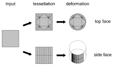
Figure 8: Patch tessellation: Top and side faces are tessellated differently since they need to undergo different deformations.
As Figure 8 shows, the actual tessellation of a patch also depends on whether the patch is part of the bottom or the side faces of the cube. Since the cube shall be tessellated into a cylinder, the side faces only need to be subdivided horizontally. A vertical subdi-vision is required by the tessellator stage. The top face generally requires high tessellation on the edges, but again one face needs to be added to the center for the tessellator. The values of the gl TessLevelInner and gl TessLevelOuter arrays are set accord-ingly. The rest of the output variables are only required once per patch. They could normally be declared as patch variables, but this caused problems on Intel HD Graphics. Thus they are passed as normal per-vertex attributes, but only the attribute at index 0 is set.
Tessellation Evaluation Shader: In the tessellation evaluation shader (TES), the newly created vertices are assigned to their final po-sitions. Therefore, the shader is invoked once per vertex. Inputs into the TES are the outputs of the TCS, aggregated into arrays. Each array entry corresponds to one of the output patch vertices of the TCS. To calculate the position of the inner vertices, the coordinates of the output patch vertices have to be interpolated. For that purpose the built-in input variable vec3 gl TessCoord provides the appropriate linear interpolation weights. For quad patches, the first two components (u and v) of the vector contain the horizontal and vertical position of the new vertex, relative to the input patch. They can be used for bilinear interpolation. For triangular patches on the other hand all three components would be used and would contain barycentric coordinates. The interpo-lated positions are then projected onto the unit circle by normal-izing their x-z-component. Depending on the type of face, the final position and the vertex normal (both in local coordinates) are calculated in the following manner:
• Top face: Here the normal is simply the normal of the cube’s face. The position of the border vertices (u and v are 0 or 1) are just their projected position. All other vertices need to lie inside the circle to prevent degenerated triangles. More formally:−→xlocal= (1−α)−→xinterpolated+α−→xprojected
withα=max(|2u−1|,|2v−1|)
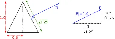
• Side face: For the tail of the glyph, the final positions are just the projected positions and the normals are simply the normalized x-z-component. For the head the procedure is a bit more complicated. The head cylinder has to be tapered to become a cone. This means that the normals are not just pointing outwards anymore, but slightly towards the tip of the arrow head. Figure 9 shows how the normal can be cal-culated from the dimensions of the cone. The y-component of the normal can directly be set to 0.5
√
1.25, while the (already normalized) x-z-component is scaled by √1.25
Figure 9: The cone’s normal is perpendicular to its surface and can be calculated from its dimensions.
Until now, all calculations were performed in local coordinates. As a final step, vertex positions have to be scaled, rotated and moved according to the instance data. The normals have to be rotated as well. After perspective projection, the glyph is ready for shading.
Fragment Shader: Since the geometry shader stage is omitted, the outputs of the TES are passed directly to the fragment shader. The fragment shader calculates a simple Phong shading using a head light (the camera position is the light position). The diffuse color of the glyph is determined by color mapping the attribute associated with the glyph.
4. CONCLUSION
In this paper we presented our approaches for the interactive vi-sualization of marine sand dune displacements within the IQmu-lus project. The described visualization techniques utilize mod-ern GPU based methods to achieve interactive rates when analyz-ing the intermediate and final results of the automatic workflow. These rates are achieved by generating the geometry which is displayed directly on the GPU. We presented two different ap-proaches, one for the rendering of LR B-Splines representing a large point cloud and second the dynamic generation of displace-ments glyphs based on results from the displacement detection workflow.
5. FUTURE WORK
The presented visualizations are currently tested and evaluated by end users within the IQmulus project and the first responses where positive. We will take the results into account to enhance the presented approaches. Furthermore, we will work on the fol-lowing topics in the future: LR B-Splines are not very well suited for representing terrains with a huge number of elements. In these cases, it will be important to develop e.g., tiling techniques. It is important that the tiled representation maintains continuity between different patches to avoid artifacts on the boundary be-tween them. Regarding the glyph visualization we will work on the exploitation of uncertainty (correlation coefficient) and the incorporation of vertical changes to get a full 3D representation of the deformation. Another interesting topic is the analysis of time-series instead of the comparison of only two timesteps.
ACKNOWLEDGEMENTS
Research leading to the results presented here is carried out within the project IQmulus (A High-volume Fusion and Analysis Plat-form for Geospatial Point Clouds, Coverages and Volumetric Data
Girod, L., 2015. MicMac, Apero and Other Beverages in a Nut-shell. ENSG - Marne-la-Valle.
Dokken, T., Lyche, T. and Pettersen, K. F., 2013. Polynomial splines over locally refined box-partitions. Computer Aided Ge-ometric Design 30(3), pp. 331–356.
Duffy, G. P. and Hughes-Clarke, J. E., 2005. Application of spa-tial cross correlation to detection of migration of submarine sand dunes. Journal of Geophysical Research: Earth Surface (2003– 2012).
Franzetti, M., Le Roy, P., Delacourt, C., Garlan, T., Cancou¨et, R., Sukhovich, A. and Deschamps, A., 2013. Giant dune mor-phologies and dynamics in a deep continental shelf environment: example of the banc du four (western brittany, france). Marine Geology 346, pp. 17–30.
Hjelmervik, J. M. and Fuchs, F. G., 2015. Interactive Pixel-Accurate Rendering of LR-Splines and T-Splines. In: B. Bickel and T. Ritschel (eds), EG 2015 - Short Papers, The Eurographics Association.
Leprince, S., Barbot, S., Ayoub, F. and Avouac, J.-P., 2007. Auto-matic and precise orthorectification, coregistration, and subpixel correlation of satellite images, application to ground deformation measurements. Geoscience and Remote Sensing, IEEE Transac-tions on 45(6), pp. 1529–1558.
Rosu, A.-M., Pierrot-Deseilligny, M., Delorme, A., Binet, R. and Klinger, Y., 2015. Measurement of ground displacement from optical satellite image correlation using the free open-source soft-ware micmac. ISPRS Journal of Photogrammetry and Remote Sensing 100, pp. 48–59.
Skytt, V., Barrowclough, O. and Dokken, T., 2015. Locally re-fined spline surfaces for representation of terrain data. Computers & Graphics.
Stumpf, A., Cancout, R., Piete, H., Delacourt, Christophe, Spag-nuolo, Michela, Cerri, Andrea, Sirmacek, Beril, Roderik and Lindenbergh, Roderik, 2014a. Change detection and dynamics toolkit. Technical Report D4.5.1, IQmulus consortium, Brest, France.
Stumpf, A., Malet, J.-P., Allemand, P. and Ulrich, P., 2014b. Surface reconstruction and landslide displacement measurements with pl´eiades satellite images. ISPRS Journal of Photogrammetry and Remote Sensing 95, pp. 1–12.
Van Landeghem, K. J., Baas, J. H., Mitchell, N. C., Wilcockson, D. and Wheeler, A. J., 2012. Reversed sediment wave migra-tion in the irish sea, nw europe: A reappraisal of the validity of geometry-based predictive modelling and assumptions. Marine Geology 295, pp. 95–112.