METRIC CALIBRATION OF A FOCUSED PLENOPTIC CAMERA BASED ON
A 3D CALIBRATION TARGET
N. Zellera, c, C.A. Nouryb, d, F. Quinta, C. Teuli`ereb, d, U. Stillac, M. Dhomeb, d a
Karlsruhe University of Applied Sciences, 76133 Karlsruhe, Germany - [email protected]; [email protected] bUniversit´e Clermont Auvergne, Universit´e Blaise Pascal, Institut Pascal, BP 10448, F63000 ClermontFerrand, France
-charles [email protected]; [email protected]; [email protected] c
Technische Universit¨at M¨unchen, Germany, 80290 Munich, Germany - [email protected] dCNRS, UMR 6602, IP, F-63178 Aubi`ere, France
ICWG III/I
KEY WORDS:Bundle adjustment, depth accuracy, depth distortion model, focused plenoptic camera, metric camera calibration
ABSTRACT:
In this paper we present a new calibration approach for focused plenoptic cameras. We derive a new mathematical projection model of a focused plenoptic camera which considers lateral as well as depth distortion. Therefore, we derive a new depth distortion model directly from the theory of depth estimation in a focused plenoptic camera. In total the model consists of five intrinsic parameters, the parameters for radial and tangential distortion in the image plane and two new depth distortion parameters. In the proposed calibration we perform a complete bundle adjustment based on a 3D calibration target. The residual of our optimization approach is three dimensional, where the depth residual is defined by a scaled version of the inverse virtual depth difference and thus conforms well to the measured data. Our method is evaluated based on different camera setups and shows good accuracy. For a better characterization of our approach we evaluate the accuracy of virtual image points projected back to 3D space.
1. INTRODUCTION
In the last years light-field (or plenoptic) cameras became more and more popular. One reason therefor is the availability of such camera systems on the market.
Plenoptic cameras capture, different from regular cameras, not only a 2D image of a scene, but a complete 4D light-field repre-sentation (Adelson and Wang, 1992, Gortler et al., 1996). Due to this additional information plenoptic cameras find usage for a variety of applications in photogrammetry as well as computer vision. Here, plenoptic cameras replace for example other depth sensors like stereo camera systems.
To use such a depth sensor for instance in photogrammetric ap-plications a precise metric calibration is mandatory. While the calibration of monocular cameras and stereo camera systems has been studied over the last decades, there is no overall accepted mathematical model available for plenoptic cameras yet. There-fore, this paper introduces a new model for focused plenoptic cameras (Lumsdaine and Georgiev, 2009, Perwaß and Wietzke, 2012) and presents how this model can be precisely determined in a metric calibration process using a 3D calibration target.
1.1 Related Work
During the last years different methods where published to cali-brate a plenoptic camera. This section lists calibration meth-ods for unfocused plenoptic cameras (Adelson and Wang, 1992, Ng et al., 2005) and focused plenoptic cameras (Lumsdaine and Georgiev, 2009, Perwaß and Wietzke, 2012) separately.
Until today the unfocused plenoptic camera is mostly used in consumer or image processing applications where a precise met-ric relation between object and image space is not mandatorily needed. Ng and Hanrahan for instance presented a method for
correcting aberrations of the main lens on the recorded 4D light-field inside the camera (Ng and Hanrahan, 2006).
In 2013 Dansereau et al. presented the first complete mathemati-cal model of an unfocused plenoptic camera (Dansereau et al., 2013). Their model consists of 15 parameters which include, be-sides the projection from object space to the sensor, the micro lens array (MLA) orientation as well as a distortion model for the main lens.
Bok et al. proposed a method which does not use point features to solve for the calibration model but line features extracted from the micro images (Bok et al., 2014).
A first calibration method for focused plenoptic cameras was posed by Johannsen et al. (Johannsen et al., 2013). They pro-posed a camera model tailored especially for Raytrix cameras which consists of 15 parameters. This model considers lateral distortion (image distortion) as well as depth distortion and shows reasonable results for the evaluated distances from36cm to50cm.
The method of Johannsen et al. was further developed by Heinze et al. and resulted in an automated metric calibration method (Heinze et al., 2015). In their method calibration is performed based on a planar object which is moved freely in front of the camera.
In a previous work, Zeller et al. focused on developing efficient calibration methods for larger object distances (>50cm) (Zeller et al., 2014). They present three different models to define the relationship between object distance and the virtual depth which is estimated based on the light-field. Besides, the calibration pro-cess is split into two parts, where the optical path and the depth are handled separately.
1.2 Contribution of this Work
main lens sensor
MLA
bL aL
(a) Keplerian configuration
main lens sensor
MLA
bL aL
(b) Galilean configuration
Figure 1. Cross view of the two possible configurations (Keple-rian and Galilean) of a focused plenoptic camera.
well as virtual depth distortion. While the model shows similarity with respect to the one in (Heinze et al., 2015) some significant changes were made which adapt the model better to the physical camera.
Firstly, we consider lateral distortion after projecting all virtual image points, which are the image points created by the main lens, back to a mutual image plane, along their central ray. In contrast, Heinze et al. apply lateral distortion directly on the vir-tual image. Thereby, we receive a model for lateral distortion which conforms better to the reality since the virtual image is not formed on a plane but on an undulating surface defined by the image distance (distance to the main lens) of each point. Besides, we show that the depth distortion can be derived from the lat-eral distortion model since in a plenoptic camera the depth map is based on disparity estimation in the raw image.
We are using a 3D target in order to obtain precise calibration parameters by performing a bundle adjustment on feature points.
In our optimization approach the depth residual is defined by a scaled version of the inverse virtual depth difference which con-forms better to the measured data.
In contrast to previous methods we show that our calibration gives good results up to object distances of a few meters. In addition, we evaluate the accuracy of points projected back to object space in 3D, which has not been done in any of the previous publica-tions.
The main part of this paper is structured as follows. Section 2 briefly presents the concept of a focused plenoptic camera. The camera model derived based on this concept is presented in Sec-tion 3. In SecSec-tion 4 we formulate the non-linear problem which is optimized to obtain the plenoptic camera model. Section 5 presents the complete calibration workflow. Section 6 evaluates the calibration based on real data and Section 7 draws conclu-sion.
2. THE FOCUSED PLENOPTIC CAMERA
Even though there exist different concepts of MLA based plenop-tic camera (Ng et al., 2005, Adelson and Wang, 1992) we will focus here only on the concept of a focused plenoptic camera (Lumsdaine and Georgiev, 2009).
As proposed by (Lumsdaine and Georgiev, 2008, Lumsdaine and Georgiev, 2009) a focused plenoptic camera can be set up in two
B bL0
b
fL bL DM
DM
DM DL
main lens sensor
MLA
Figure 2. Optical path inside a focused plenoptic camera based on the Galilean configuration.
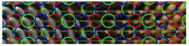
Figure 3. Section of the micro lens images (raw image) of a Raytrix camera. Different micro lens types are marked by dif-ferent colors.
different configurations. The Keplerian and the Galilean config-uration (Fig. 1). While in the Keplerian configconfig-uration MLA and sensor are placed behind the focused image created by the main lens (Fig. 1a), in the Galilean configuration MLA and sensor are placed in front of the focused main lens image (Fig. 1b). Since in the Galilean configuration the main lens image exists only as a virtual image, we will call it as such in the following.
The camera model presented in this paper was developed based on a Raytrix camera, which is a plenoptic camera in the Galilean configuration. Nevertheless, by slightly adapting the model pro-posed in Section 3 a similar calibration can be applied to cameras in the Keplerian configuration.
An image point in a micro image is composed only by a sub-bundle of all rays tracing through the main lens aperture. Con-sequently the micro images have already a larger depth of field (DOF) than a regular camera with the same aperture. In a Raytrix camera the DOF is further increased by using an interlaced MLA in a hexagonal arrangement (see Fig. 3). This MLA consists of three different micro lens types, where each type has as different focal length and thus focuses a different virtual image distance (resp. object distance) on the sensor. The DOFs of the three micro lens types are chosen such that they are just adjacent to each other. Thus, the effective DOF of the camera is increased compared to an MLA with only one type of micro lenses. In the sensor image shown in Figure 3 the blue micro images are in fo-cus while the green and red ones are blurred. Since each virtual image point is projected to multiple micro images it can be as-sured that each point is recorded in focus at least once and thus a complete focused image can be reconstructed. This also can be seen from Figure 3, where similar structures occur in adjacent micro images. For more details we refer to (Perwaß and Wietzke, 2012).
In the following part of this section we will discuss the projec-tion process in a focused plenoptic camera based on the Galilean configuration. For the main lens a thin lens model is used, while each of the micro lenses is modeled by a pinhole.
object distanceaLand image distancebLis defined dependent on the focal lengthfLby the following equation:
1
Furthermore, for each point projected from object space to image space a so called virtual depthvcan be estimated based on the disparitypxof corresponding points in the micro images (Perwaß and Wietzke, 2012). Therefor various algorithms can be used (Zeller et al., 2015, Bishop and Favaro, 2009). The relationship between the virtual depthvand the estimated disparitypxis given by the following equation:
v= b
B = d px
(2)
As one can see, the virtual depth is just a scaled version of the distancebbetween a virtual image pointpV and the plane of the MLA. In this eq. (2)Bis the distance between MLA and sen-sor andddefines the distance between the principal points of the respective micro lenses on the sensor. In general a virtual image pointpV is projected to more than two micro images (see Fig. 2) and thus multiple virtual depth observations with different base-line distancesdare received. Here,dis a multiple of the micro lens apertureDM (d = k·DM withk ≥ 1). Due to the 2D arrangement of the MLA the multiplekis not mandatory an in-teger.
3. CAMERA MODEL
This section presents the developed model for a focused plenoptic camera which will be used in the calibration process (Section 5).
The thin lens model and the pinhole model were used to repre-sent the main lens and the micro lenses respectively. In reality of course the main lens does not satisfy the model of a thin lens. Nevertheless, this simplification does not effect the overall pro-jection from object space to virtual image space.
To handle the imperfection of the main lens a distortion model for the virtual image space is defined. This model consists of lateral as well as depth distortion. One could argue that also the micro lenses add distortion to the projection. Nevertheless, since for the camera used in our research one micro lens has a very narrow field of view and only about 23 pixels in diameter, any distortion on the pixel coordinates generated by the micro lenses can be neglected.
3.1 Projection Model without Distortion
Unlike regular cameras, where a 3D object space is projected to a 2D image plane, in a focused plenoptic camera a 3D object space is projected to a 3D image space. This virtual image space is indirectly captured in the 4D light-field.
In the following derivation we will consider the object space to be aligned to the camera frame. Thus, a point in object space pOis defined by its homogeneous 3D camera coordinatesXC=
(xC, yC, zC,1)T. The camera coordinate system has its origin in the optical center of the main lens, while thez-axis is pointing towards the object (zC > 0), they-axis is pointing downwards and thex-axis is pointing to the right.
For the virtual image space we define a mirrored coordinate sys-tem, which means that all unit vectors are pointing in the opposite direction as those of the camera coordinate system. Here a virtual image pointpV is defined by the homogeneous 3D coordinates
XV = (xV, yV, zV,1)T. The virtual image coordinates have their origin on the intersection of the optical axis with the plane of the MLA. Both camera coordinatesXCas well as virtual
im-age coordinatesXV have metric dimensions.
Using the ideal thin lens model for the main lens a virtual image point, defined by the coordinatesXV, can be calculated based
on the corresponding object point coordinatesXC, as given in
eq. (3).
In eq. (3) the matrix coefficientsbLandb, which conform to the ones in Figure 2, are dependent on the object distanceaL=zC and are defined as follows:
bL=
The introduced scaling factorλis just the object distancezC:
λ=zC (6)
To receive the virtual image coordinates in the dimensions they are measuredX′
V = (x′V, yV′ , v,1) T
, a scaling of the axis as well as a translation along thex- andy-axis has to be performed (x′V andyV′ are defined in pixels), as defined in eq. (7).
Heresxandsydefine the size of a pixel, whileBis the distance between MLA and sensor.
By combining the matrixKandKSone can define the complete transform from camera coordinatesXCto virtual image
coordi-natesX′V, as given in eq. (8).
λ·X′
V =KS·K·XC (8)
Since the pixel size (sx,sy) for a certain sensor is known in gen-eral, there are five parameters left which have to be estimated. These parameters are the principal point (cx, cy) expressed in pixels, the distance between MLA and sensor B, the distance from optical main lens center to MLAbL0and the main lens
fo-cal lengthfL.
3.2 Distortion Model
Section 3.1 defines the projection from an object pointpOto the corresponding virtual image point pV without considering any imperfection in the lens or the setup. In this section we will define a lens distortion model which corrects the position of a virtual image pointpV inx,yandzdirection.
To implement the distortion model another coordinate system with the homogeneous coordinatesXI = (xI, yI, zI,1)is
de-fined. The coordinatesXIactually define the pinhole projection
the main lens with an image plane. In the presented model the image plane is chosen to be the same as the MLA plane. Thus, by splitting up the matrixKintoKIandKV (eq. (9)) the image coordinatesXIresult as defined in eq. (10).
K=KV·KI
By the introduction of image coordinatesXI we are able to
in-troduce a lateral distortion model on this image plane, similar as for a regular camera. From eq. (9) and (10) one can see that thez -coordinates in the spaces defined byXIandXV are equivalent (zI=zV).
In the following we define our distortion model, which is split into lateral and depth distortion.
3.2.1 Lateral Distortion For lateral distortion a model which consists of radial symmetric as well as tangential distortion is de-fined. This is one of the most commonly used models in pho-togrammetry.
The radial symmetric distortion is defined by a polynomial of the variabler, as defined in eq. (11).
∆rrad=A0r
Hereris the distance between the principal point and the coordi-nates on the image plane:
r=
This results in the correction terms∆xradand∆yradas given in eq. (13) and (14).
In our implementation we use a radial distortion model consisting of three coefficients (A0toA2). Besides, for tangential distortion
we used the model defined in (Brown, 1966) using only the two first parametersB0andB1. The terms given in eq. (15) and (16)
Based on the correction terms the distorted image coordinatesxId andyIdare calculated from the ideal projection as follows:
xId=xI+ ∆xrad+ ∆xtan (17) yId=yI+ ∆yrad+ ∆ytan (18)
3.2.2 Depth Distortion To describe the depth distortion a new model is defined. While other calibration methods define the depth distortion by just adding a polynomial based correction
term (Johannsen et al., 2013, Heinze et al., 2015), our goal was to find an analytical expression describing the depth distortion as a function of the lateral distortion and thus reflecting the physi-cal reality. Therefore, in the following the depth correction term
∆vis derived from the relation between the virtual depthvand the corresponding estimated disparitypx. In the following equa-tions all parameters with subscriptdrefer to distorted parameters which are actually measured, while the parameters without a sub-script are the undistorted ones resulting from the ideal projection.
Equation (19) defines, similar to eq. (2), the estimated virtual depth based on corresponding pointsxdiin the micro images and
its micro image centerscdi. Here the pixel coordinates as well as
the micro lens centers are affected by the distortion.
vd=
In general both,xdiandcdican be defined as pixel coordinates
on the sensor (in the raw image).
Due to epipolar geometry and rectified micro images, the differ-ence vectors(cd2−cd1)and(xd2−xd1)point always in the
same direction. In addition, since eq. (19) is only defined for pos-itive virtual depths,kcd2−cd1k ≥ kxd2−xd1kalways holds.
Therefore, eq. (19) can be simplified as follows:
vd=
kcd2−cd1k
kcd2−cd1k − kxd2−xd1k (20)
Replacing the distorted coordinates by the sum of undistorted co-ordinates and their correction terms results in eq. (21). Here one can assume that a micro lens centerciundergoes the same
dis-tortion∆xi as the underlying image pointxi since both have
similar coordinates.
Under the assumption that only radial symmetric distortion is present and that k∆x2k
holds, eq. (21) can be simplified as follows:
vd≈
The assumption which was made above holds well for micro lenses which are far from the principal point. For close points the distortion anyway is small and thus can be neglected. Besides, radial symmetric distortion in general is dominant over other dis-tortion terms.
From eq. (22) one obtains that the distorted virtual depthvdcan be defined as the sum of the undistorted virtual depthvand a correction term∆v, as defined in eq. (23).
∆v=±k∆x2−∆x1k px
(23)
less the same direction, eq. (23) can be approximated as follows:
and∆x1point in the same direction again holds well for large
image coordinatesxi. The radiusrdefines the distance from the
principal point to the orthogonal projection of the virtual image pointpV on the sensor plane.
To simplify the depth distortion model only the first coefficient of the radial distortionA0, defined in eq. (11), is considered to be
significant. Thus, based on eq. (11) the following definition for
∆vis received:
Replacingpxbydv(see eq. (2)) results in the following equation:
∆v=A0·v
For a virtual image pointpV with virtual depthvall micro lenses which see this point lie within a circle with diameterDM ·v around the orthogonal projection of the virtual image pointpV on the MLA plane. Thus, in first approximation the maximum baseline distance used for depth estimation is equivalent to this diameter. Therefore, we replacedbyDM·vwhich results in the final definition of our depth distortion model, as given in eq. (27).
∆v= 3A0·v·r
Since the distortion is just defined by additive terms they can be represented by a translation matrixKDas defined in eq. (28).
KD=
This matrix consists of seven distortion parameters (A0,A1,A2,
B0,B1,D0andD1) which have to be estimated in the calibration
process.
3.3 Complete Camera Model
Under consideration of the projection as well as the distortion, the complete projection from an object point in camera coordinates
XCto the corresponding virtual image point in distorted
coordi-natesX′
V d, which are actually measured, is defined as follows:
λ·X′V d=KS·KV·KD·KI·XC (29)
The projection model defined in eq. (29) consists of 12 unknown intrinsic parameters which have to be estimated during calibra-tion.
4. NON-LINEAR OPTIMIZATION PROBLEM
To estimate the camera model an optimization problem has to be define, which can be solved based on recorded reference points.
We define this optimization problem as a bundle adjustment, where the intrinsic as well as extrinsic camera parameters are estimated based on multiple recordings of a 3D target.
The relation between an object point p{Oi} with homogeneous world coordinatesX{i}
W and the corresponding virtual image point in thej-th framep{Vi,j}is defined based on the model presented in Section 3 as follows:
X′{i,j}
HereGj∈SE(3)defines the rigid body transform (special Eu-clidean transform) from world coordinatesX{i}
W to the camera coordinates of thej-th frameX{i,j}
C . Besides,λijis defined by z{Ci,j}(see eq. (6)).
In the following we will denote a virtual image pointX′V dwhich
was calculated based on the projection given in eq. (30) by the coordinatesxproj,yproj, andvproj, while we denote the corre-sponding reference point measured from the recorded image by the coordinatesxmeas,ymeas, andvmeas.
Based on the projected as well as measured points the cost func-tion given in eq. (31) can be defined.
C=
HereNdefines the number of 3D points in object space, while Mis the number of frames used for calibration. The functionθij represents the visibility of an object point in a certain frame (see eq. (32)).
θij=
(
1, ifp{Oi}is visible inj-th image,
0, if not. (32)
The vectorεijis defined as given in the following equations:
εij=ε{i,j}
The residual of the virtual depthεvis defined as given since the virtual depth vis inverse proportional to the disparity px esti-mated from the micro images (see eq. (2)) and thus the inverse virtual depth can be considered to be Gaussian distributed (as an-alyzed in (Zeller et al., 2015)). As already stated in Section 3.2.2, the baseline distancedis on average proportional to the estimated virtual depthv. Thus, the difference in the inverse virtual depth is scaled by the virtual depthvitself. The parameterwis just a constant factor which defines the weight betweenεx,εy, andεv.
5. CALIBRATION PROCESS
Raw images
Image processing / depth estimation
Totally focused image Virtual depth map
Features detection Interest points
Projection parameters initialization
Initial projection parameters
Projection parameters optimization Final projection parameters
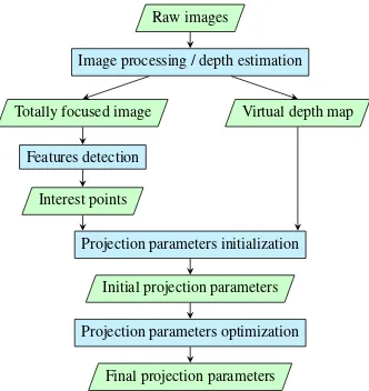
Figure 4. Flow chart of the calibration process.
5.1 Preprocessing
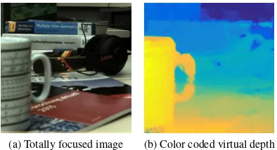
In a preprocessing step from the recorded raw images virtual depth maps are estimated as well as totally focused intensity im-ages are synthesized. For the experiments presented in Section 6.1 the algorithm implemented in the Raytrix API was used for depth estimation. Figure 5 shows an example of the input images (to-tally focused intensity image and virtual depth map) for the cali-bration process. Based on the totally focused intensity image fea-ture points of the calibration target are extracted.
5.2 Intrinsic and Extrinsic Parameters Initialization
After the preprocessing initial intrinsic and extrinsic parameters are estimated based on the feature points. Hence, we perform a bundle adjustment based on a proprietary calibration software (Aicon 3D Systems, 1990) only using the totally focused images. In the bundle adjustment a regular pinhole camera model is used. Of course this does not correspond to reality but good initial pa-rameters are received.
In that way, beside the initial extrinsic orientation for each frame (ω,φ,κ,tx,ty,tz) and the 3D points in world coordinates (Fig. 6), the intrinsic camera parameters of a pinhole camera are re-ceived. These intrinsic parameters are the principal distancef, the principal point(cx, cy), as well as radial and tangential dis-tortion parameters. In a first approximation the principal distance is assumed to be equal to the main lens focal lengthfL = f. This assumption is sufficient to receive an initial parameter for the main lens focal length.
There are still two missing parameters to initialize the plenoptic camera model. Those parameters arebL0, the distance between
the main lens and the MLA, andB, the distance between the MLA and the sensor (Fig. 2). To estimate the initial values of those two parameters, we used the physical model of the camera as explained in (Zeller et al., 2014). Here the parametersbL0and
B are received by solving the linear equation given in expres-sion (37) which is obtained from eq. (4).
bL=b+bL0=v·B+bL0 (37)
This is done by using all feature points in all recorded frames. Based on the initial value for the focal length of the main lens fLand thez-component of the camera coordinateszCthe cor-responding image distancebLis calculated using the thin lens equation (eq. (4)). Finally, based on the image distancesbL, cal-culated for all feature points, and the corresponding virtual depth
(a) Totally focused image (b) Color coded virtual depth
Figure 5. Sample image of the 3D calibration target.
Figure 6. Calibration points and camera poses in 3D object space. Camera poses are represented by the three orthogonal unit vectors of the camera coordinates.
v, received from the depth maps, the parametersB andbL0are estimated.
5.3 Optimization based on Plenoptic Camera Model
After the initialization the plenoptic camera model is solved in a non-linear optimization process. In this optimization process all intrinsic as well as extrinsic parameters are adjusted based on the optimization problem defined in Section 4. Evaluations showed, that the 3D points received from the software have sub-millimeter accuracy and therefore will not to be adjusted in the optimization.
The cost functionC, defined in eq. (31), is optimized with re-spect to the intrinsic and extrinsic parameters by the Levenberg-Marquardt algorithm implemented in the Ceres-Solver library (Agarwal et al., 2010).
6. EVALUATION
In this section we evaluate our proposed calibration method. Here, we want to evaluate on one side the validity of the proposed model and on the other side to accuracy of the plenoptic camera itself as a depth sensor.
All experiments were performed based on a Raytrix R5 camera. Three setups with different main lens focal lengths (fL= 35mm, fL= 16mm,fL= 12.5mm) were used.
6.1 Experiments
(a) Totally focused image (b) Color coded virtual depth
Figure 7. Sample scene recorded with focal lengthfL= 35mm used for qualitative evaluation.
6.1.2 Measuring Metric 3D Accuracy In a second experi-ment we evaluate the measuring accuracy of the plenoptic camera itself, using our camera model. During the calibration we were not able to record frames for an object distance closer than ap-proximately1m. For close distances the camera does not capture enough feature points to calculate meaningful statistics. Because of that reason, and since the depth range strongly decays with de-creasing main lens focal lengthfLwe were only able to record meaningful statistics for thefL= 35mm focal length.
Thus, in this second experiment we evaluate the deviation of a virtual image point, measured by the camera and projected back to 3D space, from the actual ground truth which we received from our 3D calibration object.
Therefore, based on the recorded data we calculate the 3D pro-jection error of the point with indexiin thej-th frame∆X{i,j}
C ,
as given in eq. (39).
X{i,j}
C = (KS·KV ·KD·KI·)−
1
·λij·X′{V di,j} (38)
∆X{i,j}
C =X
{i,j}
C −Gj·X {i}
W (39)
Here, X{i,j}
C is the measured virtual image pointX ′{i,j} V d pro-jected back to 3D space as defined in eq. (38), whileX{i}
W is the corresponding 3D reference point in world coordinates (ground truth).
The 3D projection error ∆X{i,j}
C is evaluated for object dis-tanceszCfrom1.4m up to5m.
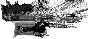
6.1.3 Calculating the Point Cloud of Real Scene In a last experiment we recorded a real scene and calculate the 3D metric point cloud out of it for a qualitative evaluation of the model. Therefore, the 3D metric point cloud was calculated for the scene shown in Figure 5 which was recorded with thefL = 35mm setup.
6.2 Results
6.2.1 Estimating the Camera Parameters Table 1 shows the resulting parameters of the estimated plenoptic camera model for all three setups (fL = 35mm, fL = 16mm, andfL =
12.5mm). As one can see, for all three focal lengths the esti-mated parameterfLis quite similar to the nominal focal length of the respective lens. The parameterB, which actually should not be dependent on the setup, stays quite constant over all setups and thus confirms the plausibility of the estimated parameters. The slight deviation in the parameterBforfL= 12.5mm prob-ably can be explained by a too short range in which the virtual depth values of the feature points are distributed. Here, recording feature points for closer object distances could be beneficial.
lens 35mm 16mm 12.5mm fL(in mm) 34.85 16.26 12.61 bL0(in mm) 34.01 15.30 11.55
B(in mm) 0.3600 0.3695 0.4654 cx(in pixel) 508.4 510.2 502.5 cy(in pixel) 514.9 523.6 520.8
Table 1. Estimated intrinsic parameters of the proposed focused plenoptic camera model for different main lens focal length.
lens 35mm 16mm 12.5mm
pinhole cam. (in pixel) 1.365 5.346 8.118 our model (in pixel) 0.069 0.068 0.078
Table 2. Comparison of the reprojection error using a pinhole camera model as well as our proposed focused plenoptic camera model for different main lens focal length.
Another indication for plausible parameters is, that to focus an image up to an object distance of infinity the condition fL ≤
2·B+bL0has to be fulfilled (see (Perwaß and Wietzke, 2012)),
which is the case for all three setups.
Furthermore, the reprojection error calculated from the feature points confirms the validity of our model. In Table 2 we compare the error for a regular pinhole camera model and for the proposed focused plenoptic camera model. As one can see, the error is im-proved by some orders of magnitude by introducing the plenop-tic camera model. One can see that for a shorter main lens focal lengthfLthe reprojection error increases. This is the case, since here the projection in the plenoptic camera stronger deviates from the pinhole camera projection.
6.2.2 Measuring Metric 3D Accuracy Figure 8 shows the RMSE between the reference points and the back projected points in 3D object space for object distances fromzC = 1.4m up to zC= 5m, using thefL= 35mm focal length. We calculated the RMSE for each coordinate separately as well as for the complete 3D error vector∆XC.
As could be expected, the error along thex- andy-coordinate is much smaller than the one inz-direction. Nevertheless, all three errors increase approximately proportional to each other with in-creasing object distancezC. This is quite obvious, since the co-ordinatesxCandyCare linearly dependent onzCand thus also effected by the depth error.
The overall error in 3D space ranges from50mm at an object distance of1.4m up to300mm at5m distance. This conforms quite well to the evaluations made in other publications as well as to the specifications given by Raytrix (see (Zeller et al., 2014)).
6.2.3 Calculating the Point Cloud of Real Scene Finally, Figure 9 shows the calculated metric point cloud for the sample scene given in Figure 7. Here one can see, that the cup which oc-curs quite large in the perspective image is scaled down to its met-ric size. Besides, the compressed virtual depth range is stretched to real metric depths.
2000 3000 4000 5000 0
10 20 30
object distancezC(in mm)
rmse
(in
mm) x-coord. (xC) y-coord. (yC)
(a) RMSE inx- andy-coordinate
2000 3000 4000 5000
0 100 200 300
object distancezC(in mm)
rmse
(in
mm)
(b) RMSE inz-coordinate
2000 3000 4000 5000
0 100 200 300
object distancezC(in mm)
rmse
(in
mm)
(c) RMSE in 3D space
Figure 8. RMSE of feature points projected back to 3D object space.
Figure 9. 3D metric point cloud of a sample scene (Fig. 7) calcu-lated based on our focused plenoptic camera model.
7. CONCLUSION
In this paper we presented a new model for a focused plenoptic camera as well as a metrical calibration approach based on a 3D target. Different to priorly published models we consider lens distortion to be constant along a central ray through the main lens. Besides, we derived a depth distortion model directly from the theory of depth estimation in a focused plenoptic camera.
We applied our calibration to three different setups which all gave good results. In addition we measured the accuracy of the focused plenoptic camera for different object distances. The measured accuracy conforms quite well to what is theoretically expected.
In future work we want to further improve our calibration ap-proach. On one hand our calibration target has to be adapted to be able to get feature points for object distances closer than1m. Besides, a denser feature point pattern is needed to reliably esti-mated depth distortion.
ACKNOWLEDGEMENTS
This research is funded partly by the Federal Ministry of Edu-cation and Research of Germany in its program ”IKT 2020
Re-search for Innovation” and partly by the French government re-search program ”Investissements d’avenir” through the IMobS3 Laboratory of Excellence (ANR-10-LABX-16-01) and the FUI n◦17 CLEAN Robot.
REFERENCES
Adelson, E. H. and Wang, J. Y. A., 1992. Single lens stereo with a plenoptic camera.IEEE Trans. on Pattern Analysis and Machine Intelligence14(2), pp. 99–106.
Agarwal, S., Mierle, K. and Others, 2010. Ceres solver. http://ceres-solver.org.
Aicon 3D Systems, 1990. Aicon 3d studio. http://aicon3D.com.
Bishop, T. E. and Favaro, P., 2009. Plenoptic depth estimation from multiple aliased views. In: IEEE 12th Int. Conf. on Com-puter Vision Workshops (ICCV Workshops), pp. 1622–1629.
Bok, Y., Jeon, H.-G. and Kweon, I., 2014. Geometric calibra-tion of micro-lens-based light-field cameras using line features. In: Computer Vision - ECCV 2014, Lecture Notes in Computer Science, Vol. 8694, pp. 47–61.
Brown, D. C., 1966. Decentering distortion of lenses. Pho-togrammetric Engineering32(3), pp. 444–462.
Dansereau, D., Pizarro, O. and Williams, S., 2013. Decoding, calibration and rectification for lenselet-based plenoptic cameras. In: IEEE Conf. on Computer Vision and Pattern Recognition (CVPR), pp. 1027–1034.
Gortler, S. J., Grzeszczuk, R., Szeliski, R. and Cohen, M. F., 1996. The lumigraph. In: Proc. 23rd Annual Conf. on Com-puter Graphics and Interactive Techniques, SIGGRAPH, ACM, New York, NY, USA, pp. 43–54.
Heinze, C., Spyropoulos, S., Hussmann, S. and Perwass, C., 2015. Automated robust metric calibration of multi-focus plenop-tic cameras. In: Proc. IEEE Int. Instrumentation and Measure-ment Technology Conf. (I2MTC), pp. 2038–2043.
Johannsen, O., Heinze, C., Goldluecke, B. and Perwaß, C., 2013. On the calibration of focused plenoptic cameras. In:GCPR Work-shop on Imaging New Modalities.
Lumsdaine, A. and Georgiev, T., 2008. Full resolution lightfield rendering. Technical report, Adobe Systems, Inc.
Lumsdaine, A. and Georgiev, T., 2009. The focused plenoptic camera. In: Proc. IEEE Int. Conf. on Computational Photogra-phy (ICCP), San Francisco, CA, pp. 1–8.
Ng, R. and Hanrahan, P., 2006. Digital correction of lens aber-rations in light field photography. In:Proc. SPIE 6342, Interna-tional Optical Design Conference, Vol. 6342.
Ng, R., Levoy, M., Br´edif, M., Guval, G., Horowitz, M. and Han-rahan, P., 2005. Light field photography with a hand-held plenop-tic camera. Technical report, Stanford University, Computer Sci-ences, CSTR.
Perwaß, C. and Wietzke, L., 2012. Single lens 3d-camera with extended depth-of-field. In:Proc. SPIE 8291, Human Vision and Electronic Imaging XVII, Burlingame, California, USA.
Zeller, N., Quint, F. and Stilla, U., 2014. Calibration and accu-racy analysis of a focused plenoptic camera. ISPRS Annals of Photogrammetry, Remote Sensing and Spatial Information Sci-encesII-3, pp. 205–212.