Conference paper

(1)

P.Walczykowski a, A.Orych a *, A.Jenerowicza, P.Karcz b

a

Department of Remote Sensing and Photogrammetry, Geodesy Institute, Faculty of Civil Engineering and Geodesy, Military University of Technology, Warsaw, Poland - (aorych, pwalczykowski, ajenerowicz)@wat.edu.pl

b

Laboratorium Badawcze ZENIT, Gdynia, Poland, pawel.karcz@zenit24.pl

Remote sensing, Acquisition, Processing, Calibration, Sensor, Error, Spectral

The paper describes a series of experiments conducted as part of the IRAMSWater Project, the aim of which is to establish methodologies for detecting and identifying pollutants in water bodies using aerial imagery data. The main idea is based on the hypothesis, that it is possible to identify certain types of physical, biological and chemical pollutants based on their spectral reflectance characteristics. The knowledge of these spectral curves is then used to determine very narrow spectral bands in which greatest reflectance variations occur between these pollutants. A frame camera is then equipped with a band pass filter, which allows only the selected bandwidth to be registered. In order to obtain reliable reflectance data straight from the images, the team at the Military University of Technology had developed a methodology for determining the necessary acquisition parameters for the sensor (integration time and f-stop depending on the distance from the scene and it's illumination). This methodology however is based on the assumption, that the imaging sensors have a linear response. This paper shows the results of experiments used to evaluate this linearity.

* Agata Orych - aorych@wat.edu.pl

!"#$ % & %'$%# % (

A team of specialists from the Department of Remote Sensing and Photogrammetry from the Military University of Technology in Warsaw have been leading a project entitled “IRAMSWater - Innovative remote sensing system for the monitoring of pollutants in rivers, offshore waters and flooded areas” (PBS1/B9/8/2012) financed by the polish National Centre for Research and Development. The main aim of the project is to create a remote sensing system based on a wide range of sensors for evaluating, identifying and determining the distribution of biological, physical and chemical pollutants in water in real time. These analyses are being conducted based on spectral characteristics of a wide selection of pollutants, based on imagery acquired in narrow bands of the electromagnetic spectrum. To ensure that these spectral reflectance coefficients are determined precisely it was essential to establish a precise methodology for obtaining these data. In international literature, the most common approach is to acquire such imagery first ensuring that each scene contains at least one reference panel with a well know spectral characteristic, and then transforming the imagery and calculating the spectral response curves during post-processing. The research team from the Military University of Technology had proposed a method of extracting precise reflectance coefficients without the need for using a reference panel on the scene. This is done by precisely determining the camera exposure parameters in controlled conditions. This method however assumes that the sensor transfer function is linear. (Huang , 2014; Bockaert, 2014).

) % # " %*

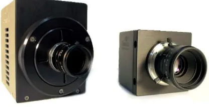
An attempt was made to determine these methodologies for acquiring spectral reflectance coefficients from two Xenics frame sensors, which record imagery in the infrared range (900-1700nm): Xeva-4246, and XEVA XS-1.7.320.

Figure 1. Xeva-4246, and XEVA XS-1.7.320

Both sensors have 320-256Px InGaAs arrays with 30 m pixels. The main difference between the sensors is the fact that the Xeva-4246 is thermo-electrically cooled (TE1) whilst the other is not (Scientific brochure Xeva-1.7-320 and XS-1.7-320, 2014). During these experiments both sensors were equipped with fixed 16mm focal length lenses with the f-stop also fixed to 16. Image acquisition was conducted in Xeneth software supplied by the manufacturer. The manufacturer also supplied calibration files for these sensors. These however were not used in this research as utilising these files greatly limits the exposure times which can be set in the software. In fact, in the case of the XEVA XS-1.7.320 sensor this parameter is not editable when

The International Archives of the Photogrammetry, Remote Sensing and Spatial Information Sciences, Volume XL-1, 2014 ISPRS Technical Commission I Symposium, 17 – 20 November 2014, Denver, Colorado, USA

This contribution has been peer-reviewed.

(2)

calibration files are used. Such settings were unacceptable to us, seeing as our methodology was to be based solely on manipulating the exposure time depending on the illumination of the scene. When defining the process of calibrating a sensor as the measurement of the output of a sensor in response to an accurately known input, then as a result of our measurements, we in fact get an equation which calibrates our images to obtain spectral reflectance characteristics.

) +! ,

) !#%- .#/ %'$%# % (

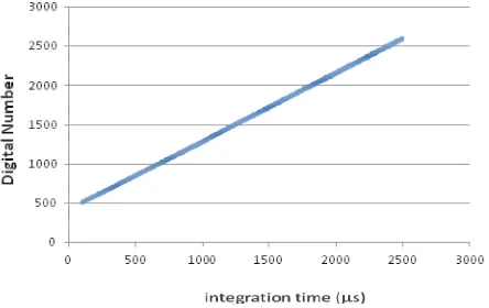
Preliminary results obtained by the Xeva-4246 sensor showed that the proposed approach is correct and gives results within ±3% of actual spectral reflectance coefficients determined using a spectroradiometer. The results of these experiments had been described in more detail in "Using XEVA video sensors in acquiring spectral reflectance coefficients", Walczykowski , 2014.

Figure 2. Image digital value (output) versus the integration time at a constant scene illumination (input) for the XEVA

4246

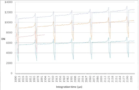
However, when conducting the same measurements using the second sensor, the XEVA XS-1.7.320, these accuracies were much lower during some, not all, conducted experiments. The results of single measuring sessions were sometimes over 10% different in comparison to reference data. There were however measurements during which accuracies around 2-3% were obtained. Having checked all other possibilities, it became evident that these inconsistencies occurred when certain specific integration times were set on the camera. This lead us to conduct a new experiment to check the transfer function of the sensor. A properly functioning sensor should have a linear (or close to linear) transfer function, meaning that an output is directly proportional to the input over its entire range so that the slope of a graph of output versus input describes a straight line (Huang , 2014; Bockaert, 2014). The image below represents a graph of the image digital value (output) versus the integration time at a constant scene illumination (input):

Figure 3. Image digital value (output) versus the integration time at a constant scene illumination (input) for the XEVA

XS-1.7.320.

As is evident from the graph above, the sensor does not have a linear transfer function. There are certain integration times, occurring periodically, which give incorrect DN values.

) ) ,. %'$%# % (

We conducted subsequent four similar experiments to determine whether this pattern is recurrent and whether the visible errors in DN - DN are constant or dependant on the light intensity and composition.

Because the preliminary experiments were very time consuming, we decided to conduct further experiments on a much narrower range of integration times (1750-2250 s). These experiments were conducted in controlled laboratory conditions, with scene irradiance measurements taken at equal intervals during the experiment (at 1800µs, 1900µs, 2000µs, 2100µs and 2215µs). The same experiment was conducted 4 times using four different scene illuminations:

• Measurement series 1 - 4,28x10-3 Watt/m2 only light source was the one used to illuminate the scene in a controlled way. We used ASD Pro Lamp illumination sources, as they are characterised by a very stable flux. Additionally, to lessen the effects of backscattering from the lamps themselves, all measurements were taken through a curtain, so that only the object of interest (the white reference panel) was visible. The distances between the light sources and white reference panel varied between the four experiments to provide the four different scene illuminations. These were measured using an ASD FieldSpec 4 spectrometer. The laboratory set up for the experiments was as follows:

(3)

Figure 4. Experiment set-up

0

An analysis of obtained results shows that there is a repeatability in the DN errors for chosen integration times for the given sensor. For each measurement series the local maximum DN erroneous values occurred at 1810, 1874, 1938, 2002, 2066, 2130, 2194 [ s], whereas the local minimum DN erroneous values were observed at 1805, 1869, 1933, 1997, 2061, 2125, 2189 [ s]. All four experiments showed that these problems occur in cycles of 64 s. Figure 5 perfectly shows the repeatability of these errors:

Figure 5. DN values of one sample obtained at different integration times. Four measurements at four different scene

illuminations

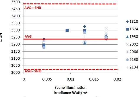
As is apparent in Figure 5, as expected, there is a strong correlation between the scene illumination and the DN values. The graph also suggests that the amplitude of the errors in DN values at specific integration times ( DN) is not affected by the scene illumination. In order to calculate the DN values for each integration time we calculated the expected pixel values at each integration time based on regression functions for each illumination. This resulted in obtained DN values, which show how much the incorrect DN values differ from the expected values. A graphical representation of these results is shown in Figure 6.

Figure 6. Errors in DN values ( DN) obtained during four experiments at four different scene illuminations.

Further calculations has shown, that independent from the scene illumination, the errors in DN values occurring at specific integration times are always constant in their values. The table below shows the DN values, calculated as the difference between the measured and theoretical DN values, for two chosen integration time ranges (marked with a circle in Figure 6).

Table1

DN values for two chosen integration time ranges (1866-1874 s and 2058-2066 s)

Time [ s]

Exp1 Exp2 Exp3 Exp4 Exp(1-4)

DN DN DN DN AVG DN

1866 -325 -293 -289 -307 _-303

1867 -396 -401 -389 -398 -396

1868 -620 -654 -624 -612 -628

1869 -867 -902 -822 -822 -853

1870 2039 2021 2086 2094 ₂₀₆₀

1871 2118 2201 2203 2173 ₂₁₇₄

1872 2410 2363 2423 2393 2397

1873 2619 2636 2713 2704 2668

1874 3195 3300 3297 3249 3260

2058 -311 - -264 -328 _-301

2059 -446 - -441 -442 -443

2060 -640 - -687 -663 -663

2061 -925 - -875 -840 -880

2062 2014 - 2073 1988 ₂₀₂₅

2063 2136 - 2167 2165 ₂₁₅₆

2064 2317 - 2448 2444 2403

2065 2587 - 2712 2686 2662

2066 3230 - 3224 3282 3246

This relationship can be also seen in Figure 7, which shows the DN values for all local maximum error values in the measured range of integrations times. These maximum errors occur at 1810, 1874, 1938, 2002, 2066, 2130, 2194 [ s], so at every 64th image (integration time).

(4)

Figure 7. DN errors for every 64th image.

All DN errors occurring on images acquired with this sensor are repeated every 64 samples and, taking into account that they vary by less than the sensor SNR (250DN), can be considered constant in their value.

The purpose of this paper was to determine the linearity of the XEVA XS-1.7.320 infrared sensor. When comparing the DN values obtained from all images in the 1750-2250ms range of integration times, a visible pattern forms. Every 64th image (integration time) is characterized by the same errors. These errors are not dependant on the scene illumination as they vary only by 0,1%-0,2%, which is much smaller than the sensors SNR (250DN), so it can be said that they are constant in value. Knowing these values it is possible to introduce simple algorithms into the image post processing stage, in order to correct these data. Taking into account that the lowest possible integration time, which according to manufacturer recommendations, should not be greater than 100 s, the first integration time which would require image corrections is 138 s. Because the pattern of errors is recurrent and repeats every 64 images, the images acquired at (138+64) s, (138+128) s...(138+64n) s will all require the same correction value in order to obtain correct DN values. Table 2 presents the values, by which acquired DN values have to be corrected for each integration time.

Table 2

Correction values for DN obtained from imagery acquired at given integration times

,

The presented article is part of research work carried out in the “Innovative remote sensing system for the monitoring of pollutants in rivers, offshore waters and flooded areas“ project- PBS1/B9/8/2012 financed by the polish National Centre for Research and Development NCBiR.

Bockaert, V., 2014, Sensor Linearity,

, http://www.dpreview.com/glossary/camera-system/sensor-linearity (25 Sep. 2014)

Huang, X., Zhang, Z.,2014, A high sensitivity and high linearity pressure sensor based on a peninsula- structures diaphragm for

low- pressure ranges A 216

(2014) 176–189

Walczykowski, P., Orych, A., Jenerowicz, A., 2014, Using XEVA video sensors in acquiring spectra reflectance

coefficients, ! "#

# $ 22-23.05.2014

Scientific brochure Xeva-1.7-320,

http://www.xenics.com/documents/XB-003_04_Xeva-1.7-320_Scientific_LowRes.pdf (20 Sep. 2014)

Scientific brochure XS-1.7-320,

http://www.xenics.com/documents/XB-001_03__XS-1.7-320_Scientific_LowRes.pdf (20 Sep. 2014)