AN ISVD-BASED EUCLIDIAN STRUCTURE FROM MOTION FOR SMARTPHONES
A. Masieroa,∗, A. Guarnieria, A. Vettorea, F. Pirottia
aInterdepartmental Research Center of Geomatics (CIRGEO), University of Padova, Viale dellUniversit 16, Legnaro (PD) 35020, Italy
(alberto.guarnieri, antonio.vettore, francesco.pirotti)@unipd.it
Commission V WG 4
KEY WORDS:Reconstruction, Georeferencing, Calibration, Camera, Real-time, Photogrammetry
ABSTRACT:
The development of Mobile Mapping systems over the last decades allowed to quickly collect georeferenced spatial measurements by means of sensors mounted on mobile vehicles. Despite the large number of applications that can potentially take advantage of such systems, because of their cost their use is currently typically limited to certain specialized organizations, companies, and Universities. However, the recent worldwide diffusion of powerful mobile devices typically embedded with GPS, Inertial Navigation System (INS), and imaging sensors is enabling the development of small and compact mobile mapping systems.
More specifically, this paper considers the development of a 3D reconstruction system based on photogrammetry methods for smart-phones (or other similar mobile devices). The limited computational resources available in such systems and the users’ request for real time reconstructions impose very stringent requirements on the computational burden of the 3D reconstruction procedure.
This work takes advantage of certain recently developed mathematical tools (incremental singular value decomposition) and of pho-togrammetry techniques (structure from motion, Tomasi–Kanade factorization) to access very computationally efficient Euclidian 3D reconstruction of the scene.
Furthermore, thanks to the presence of instrumentation for localization embedded in the device, the obtained 3D reconstruction can be properly georeferenced.
1. INTRODUCTION
The developments of photogrammetry during the last decades al-lowed to obtain high resolution 3D models of the reality from (quite low cost) camera measurements by means of well known and typically quite computational demanding signal processing procedures (data association and structure from motion methods). Despite some issues (e.g. related to the illumination conditions of the scene) may occur, the quality of the 3D reconstructions ob-tained by means of photogrammetry methods are typically com-parable with those obtained by means of other, more expensive, sensors.
Nowadays, the world-wide capillary diffusion of low cost mo-bile cameras and smartphones and the users’ demand for 3D aug-mented reality systems, possibly quickly obtained by using mo-bile devices, are motivating the development of computationally efficient 3D reconstruction methods.
This work deals with the development of a 3D reconstruction sys-tem based on measurements from an uncalibrated camera, typi-cally embedded in a (usually low cost) smartphone. In addition, the goal is to obtain a georeferenced 3D model by exploiting the measurements of a proper navigation system based on both GPS and the inertial navigation system of the smartphone.
The main challenge in the development of such 3D reconstruction systems is the reduction of the computational efforts requested by classical methods for 3D reconstruction from uncalibrated cam-eras. Recently, some methods have been proposed in the litera-ture to reduce such computational effort: most of them are based on the optimization of bundle adjustment methods, e.g. the use
∗Corresponding author.
of Preconditioned Conjugate Gradients to speed up the bundle ad-justment optimization (Agarwal et al., 2010, Byr¨od and Astr¨om, 2010).
Differently from such methods, this work takes advantage of the Incremental Singular Value Decomposition (ISVD (Brand, 2002)) to obtain a fast factorization of the measurement matrix (Tomasi and Kanade’s factorization (Tomasi and Kanade, 1992)). This procedure, which has been recently proposed by Kennedy et al. (Kennedy et al., 2013), allows to quickly obtain a projective re-construction of the scene.
This paper proposes the integration of the above factorization al-gorithm with the information provided by the navigation system embedded in the device in order to obtain a fast and effective georeferenced reconstruction of the Euclidian 3D structure of the scene: thanks to the use of computationally efficient methods, the overall reconstruction procedure can be executed in real time on standard mobile devices, e.g. smartphones.
Since the proposed procedure allows to obtain georeferenced 3D reconstructions, the outcomes of this method can be used both as reconstructions for an imaging system, and as feedback informa-tion for the navigainforma-tion system in order to improve its localizainforma-tion.
2. SYSTEM DESCRIPTION
This work assumes the use of a (typically low cost) mobile de-vice (e.g. a smartphone). Such dede-vice has to be provided of an imaging sensor (i.e. a camera), and of a navigation system.
Motion (SfM) approach (Hartley and Zisserman, 2003, Ma et al., 2003). The device is moved on several locations, where the user takes shots of the scene by means of the camera embedded in the device. 3D reconstruction is accessed by relating with each others features in shots taken from different point of views.
Nowadays, most of the cameras mounted on standard smarthones have a resolution of several Mega-pixels, usually sufficient to pro-vide accurate 3D reconstructions. Hence, the proposed approach does not impose specific requirements on the camera characteris-tics.
However, SfM methods allow to reconstruct the scene up to a scale factor (Hartley and Zisserman, 2003, Fusiello, 2000, Chiuso et al., 2000), then information on the device position provided by the navigation system has to be exploited in order to estimate the unknown scale factor and the georeferenced spatial position. Out-doors the GPS system can be sufficient to provide estimations of the device position (Piras et al., 2010), however indoors the GPS signal is usually not available (or not reliable). In order to allow position estimation in indoors conditions, the considered device is assumed to be provided of an INS based on embedded sensors as well: in particular, the considered smartphone is assumed to be provided of a 3-axis accelerometer and of a 3-axis magnetome-ter. Simultaneous measurements by such instruments allow the estimation of both the movements of the mobile device, and the attitude of the device during the camera shot.
Information on the position and the attitude of the device can be exploited in the SfM algorithms as initial conditions for iterative optimization methods of the parameters, in order to speed up the convergence. Furthermore, they can be used to reduce the bur-den of the image processing step by allowing a smart selection of images to be analyzed in order to find matched features.
Outdoor localization based on the use of the GPS signal can be considered as a quite standard procedure. Instead, several algo-rithms have been recently proposed in the literature in order to access indoor position estimation based on the combined use of different sensors (Azizyan et al., 2009, Bahl and Padmanabhan, 2000, Cenedese et al., 2010, Foxlin, 2005, El-Sheimy et al., 2006, Guarnieri et al., 2013, Lukianto and Sternberg, 2011, Masiero et al., 2013, Ruiz et al., 2012, Youssef and Agrawala, 2005, Wang et al., 2012, Widyawan et al., 2012). In the procedure described in the following section it is assumed that estimations of the device position and attitude are available. In our current implementation the positioning system is as in (Masiero et al., 2013), however different choices can be considered without affecting the effec-tiveness of the procedure.
Our current implementation of the system is on a low cost mobile phone, shown in Fig. 1. The developed application shall be exe-cuted on most the Android phones (with the above specifications on the embedded sensors).
3. ITERATIVE RECONSTRUCTION
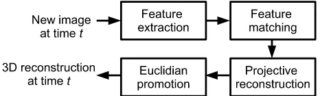
The reconstruction procedure is assumed to process data itera-tively: when a new image shoot is available a new iteration of the reconstruction procedure starts. Each iteration of the reconstruc-tion process can be decomposed in the following steps (Fig. 2) that will be detailed in the following subsections: feature extrac-tion and matching, projective reconstrucextrac-tion and Euclidian pro-motion.
Figure 1: Smartphone used to test the reconstruction system: Huawei U8650 Sonic.
Figure 2: Reconstruction procedure scheme.
3.1 Feature extraction and matching
The considered procedure relies on a feature based approach for 3D reconstruction: the geometry of the scene is reconstructed by analyzing the position of features from different point of views. In order to properly estimate the geometry of the scene the same spatial point has to be recognized and matched in the images where it is visible. Hence the use of a proper feature extraction and matching technique is of fundamental importance in order to ensure the effectiveness of the reconstruction procedure.
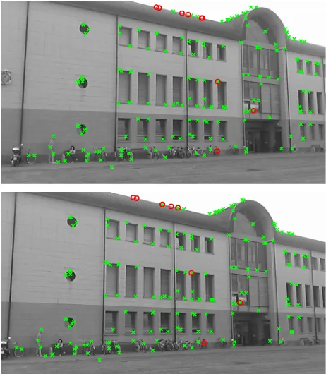
Feature extraction and matching here is decomposed in a two step procedure: first, feature extraction has been implemented by means of the Affine Scale-Invariant Feature Transform (ASIFT) (Morel and Yu, 2009): ASIFT provides a method for reliable fea-ture matching among different images. Feafea-ture matching based on ASIFT is based on the appearance of the 2D images: since images are taken from different point of views the same feature can undergo certain appearance changes, the goal of the ASIFT method is that of extracting features invariant to such deforma-tions, that are locally modeled as affine transforms.
In principle, features detected in a new image should be matched with the features of all the other frames. However, as the number of images increases such procedure becomes computationally de-manding. Several techniques based on different similarity mea-sures have been previously proposed in the literature to match features only for “highly correlated” images (Furukawa et al., 2010, Goesele et al., 2007, Masiero and Cenedese, 2013). The ra-tionale among such image selection methods is that images to be compared should be reasonably similar to have a large number of common features, however they should also have different point of views (e.g. a large baseline) to ensure a good reconstruction of the feature spatial positions. In this paper we take advantage of the information on the device position and orientation to select the small set of images to compare with the current one for fea-ture matching: the selection is done using considerations on the expected reconstruction error modeled similarly to (Masiero and Cenedese, 2013).
Figure 3: Feature extraction: example of features matched by means of the ASIFT method in two images. Features considered as properly matched after the execution of the RANSAC algo-rithm are shown as green circles. Mismatches are shown as red circles.
3.2 Projective reconstruction based on ISVD
This subsection presents a projective reconstruction procedure based on the ISVD (Brand, 2002). The approach is similar to that in (Kennedy et al., 2013), however while the work in (Kennedy et al., 2013) was limited to affine cameras, here projective cam-eras are considered. Furthermore, the projective reconstruction obtained in this subsection will be generalized to an Euclidian reconstruction and georeferenced in the next subsection.
Since the camera embedded in the mobile device is modeled as a projective camera, then the measurementmijof featurejon the
image plane of camera viewican be related with its correspond-ing 3D pointMjas follows:
mijξij=PiMj (1)
wherePi is the projective matrix of camera viewi(taking into
account also of the camera focal length), ξij is the distance of
the optical center of the camera in viewifrom the orthogonal projection ofMjon the line corresponding to the optical axis of
camera in viewi.mijandMjare written by using homogeneous
coordinate notation (Ma et al., 2003).
The above equation can be generalized for the case ofmdifferent views andnfeature points:
m11ξ11 . . . m1nξ1n
..
. ...
mm1ξ11 . . . mmnξ1n
=
P1 .. .
Pm
[
M1. . . Mn
]
(2)
where all the features are assumed to be visible in the views. By construction, matricesM andPhave rank≤4(however when estimated by real data this condition is usually not exactly satis-fied because of the presence of noise). (2) is also referred to as the Tomasi and Kanade’s factorization (Tomasi and Kanade, 1992).
Let the measurement matrixW be defined as the matrix on the left side of equation (2). Then, the rationale of (2) is that as long as the measurement matrixWis formed (and the values of theξij
are known) then the values of the projective matrices associated to camera views and the positions of the feature points can be estimated by means of the factorization ofW, e.g. by using the Singular Value Decomposition (SVD):
W=U SV⊤, P =U S(:,1 : 4), M=V(:,1 : 4)⊤, (3)
where we have used Matlab–like notation for the matrix indices. Notice that matricesPandMare estimated up to a nonsingular matrixT, i.e.
W =P M= (P T)(T−1
M). (4)
Notice that the above equation justifies also the arbitrary defini-tion ofPandMin (3).
While being very intuitive, the estimation of camera projection matrices and point positions with (2) have some drawbacks:
• First, the values of{ξij} are usually not exactly known.
Nevertheless, the information about camera positions and orientations provided by the navigation system provide us with a usually quite good initial estimate of such values: then, a more reliable estimation can be obtained by iterat-ing the estimation step ofPandMdescribed above, and an estimation step of the{ξij}from the estimatedPandM.
• The computational complexity for computing the SVD of theWmatrix (with size(3m)×n) is approximativelyO(nm2), wheren ≥ (3m). When dealing with a large number of camera views and of feature points such computational cost can become prohibitive for the considered real-time appli-cation.
Nevertheless, an iterative approach can be considered in order to tackle the last two of the above drawbacks: when a new image is available a new iteration of the algorithm for the estimation ofP
andMis started. In order to reduce the computational complex-ity of such iteration, the new solution is computed as an update of the previous solution, e.g. the new iteration is initialized by means of the previously estimated projection matrices and recon-structed feature points. A brief review of the updating rule of the ISVD will be presented in the following, for a more detailed description the reader is referred to (Brand, 2002).
LetWtbe the matrix decomposed aftertiterations of the
algo-rithm (e.g. that formed by the measured features extracted byt
views), then:
Wt≈UtStVt⊤ (5)
whereUtandVthavehcolumns (typically4≤h≤rank(Wt)).
At the(t+ 1)-th iteration, letWt+1= [Wtwt+1]wherewt+1is a proper column vector. Then, the (approximate) factorization of
Wt+1can be obtained as follows:
Wt+1= [Wt|wt+1] ≈ [UtStVt|wt+1] (6)
t stands for the pseudo-inverse
ofUt,Ut†=U
⊤
t for unitaryUt) andrt+1=wt+1−Utvt+1.
Rearranging the above equation it immediately follows that:
Wt+1≈
be factorized by the SVD
algo-rithm as follows:
Notice that the above considerations can be easily extended to the case whereWt+1is formed by adding a row toWt.
The procedure described above allow to conveniently update the SVD factorization (and consequently the factorization of (2) in our case) inO(nh2)
(form < nandhsmall with respect to
bothnandm). Since in the case of interesth≪ m, then the ISVD allow to obtain a great speed up with respect to the direct use of the SVD.
Accordingly with the definition of theW matrix, adding a col-umn or a row toWtcorresponds to add a new feature point or a
new camera view, respectively. Hence, the use of the ISVD al-lows to reduce the computational effort needed to recompute the estimation ofPandMwhen a new camera view or a new feature point are considered.
In order to deal with a feature point not available in all the camera views, when a new measurement of it is available one can select the part of theW matrix corresponding to the views where such point is visible, and update such part with a procedure similar to that presented above (slightly adapted to take into account of the different conditions of use).
The procedure described above provides an efficient iterative fac-torization method of the measurement matrixW that leads to a projective reconstruction of the scene.
3.3 Euclidian promotion and georeferencing the system
Accordingly to (4), the projective reconstruction of the scene es-timated as in the previous subsection differs from an Euclidian reconstruction for a nonsingular matrixT. Furthermore, the fi-nal goal of our system is that of obtaining a georeferenced re-construction, that differs from an Euclidian reconstruction for a translation, a rotation and a scale factor.
Two alternative approaches can be considered in order to compute a georeferenced reconstruction from the projective one.
In the first option, a two step procedure can be considered: first, estimate the Euclidian reconstruction (Euclidian promotion), and then use the estimated device positions to estimate the proper scale, translation and rotation that leads to the georeferenced re-construction.
Several procedures have been proposed in the literature to tackle the Euclidian promotion problem (Hartley and Zisserman, 2003, Fusiello, 2000). For instance, the approach based on Kruppa’s constraints described in (Heyden and Astr¨om, 1996) can be adopted. Without loss of generality (Heyden and Astr¨om, 1996, Fusiello, 2000),T can be assumed to be as follows:
T=
whereKis the intrinsic parameter matrix (Ma et al., 2003), andr
is a3×1vector. Then, the estimates{Pˆi}i=1,...,mof the camera
projective matrices obtained from the projective reconstruction have to satisfy the following constraints
ˆ a sufficiently large number of camera views are available, and camera measurements are not ideal (i.e. corrupted by noise), then the above equation typically do not have an exact solution. Then, matrixT is usually estimated by minimizing the sum of the squared differences between the left and right sides in (14) for
i= 1, . . . ,m. Such solution is usually computed by means of iterative optimization methods (e.g. Gauss–Newton algorithm).
Since the goal of the procedure is to compute a georeferenced reconstruction, here an alternative approach can is considered, i.e. the direct estimation of the transform matrixTg from the
coordinate system of the projective reconstruction to that of the georeferenced reconstruction.
Letxi be the (georeferenced) position of the device during the
i-th camera acquisition, estimated by the navigation system. The estimatexiof the device position is assumed to be affected by a
zero-mean Gaussian error with covarianceσ2
i. From a statistical
point of view, the estimation error is assumed to be isotropically distributed over the three spatial directions.
LetCibe the optical center of the camera during thei-th
acqui-sition, estimated by means of the projective reconstruction.
Assuming that the distance between the optical centers of the em-bedded camera and the point of the device used for the georefer-enced position is negligible, thenxi and Ci can be related as
follows:
xi≈TgCi , for i= 1, . . . ,m. (15)
When a quite large number of camera views is available and cam-era measurements are quite accurate, then it can be assumed that errors on the estimated optical centers{Ci}i=1,...,mare smaller
with respect to those on the device positions{xi}i=1,...,m. In
accordance with this observation, hereafter it is assumed that the errors on the estimated optical centers are negligible with respect to those on the estimated device positions. Under this assumption the matrixTgcan be effectively estimated as follows:
Tg=XΣ−
1
x C
⊤
(CΣ−x1C)
†
(16)
whereXandCare the matrices formed by collecting the vectors {xi}i=1,...,m and{Ci}i=1,...,m, respectively. Furthermore, the
matrixΣxis the covariance matrix of the first component of the
estimates{xi}, i.e. if such estimates are independent thenΣxis
a diagonalm×mmatrix. If the estimation errors on the device positions have the same variance3σ2
(equally distributed over the 3 spatial directions), thenΣx=diag(σ2, . . . , σ2).
Since the estimation error on the device position has been as-sumed to be isotropic, thenΣxis the covariance matrix for the
second and third component of the estimates{xi}, as well.
4. RESULTS AND CONCLUSIONS
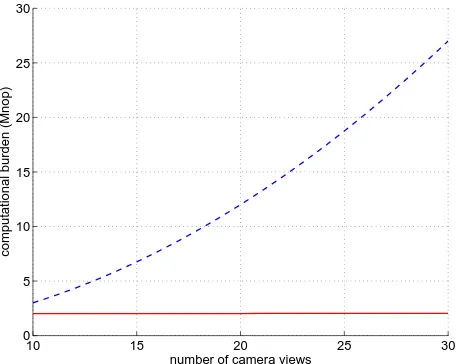
Thanks to use of the ISVD algorithm the proposed reconstruction procedure allows to significantly reduce the computational time required for computation 3D reconstructions of the scene. The system is assumed to immediately process a newly acquired im-age, first computing the image features, and then computing an updated scene 3D reconstruction. The computation of such 3D reconstruction is based on the use of the ISVD algorithm, which exploits the previously computed reconstruction in order to re-duce its computational burden: as shown in Fig. 4, as the number of camera views increases the computational load of the ISVD algorithm quickly becomes much lower than that of the SVD.
It is worth to notice that some issues may occur when adding new points to the Tomasi and Kanade’s factorization (solved by means of the ISVD as presented in subsection 3.2): for instance, the point position cannot be computed if it is not visible by some
10 15 20 25 30
0 5 10 15 20 25 30
number of camera views
computational burden (Mnop)
Figure 4: Comparison of the computational complexity (ex-pressed in number of operations (nop) of one iteration of the SVD (blue dashed line) and of the ISVD (red solid line) for a matrix
W with size3m×n.
cameras. Hence, a measurement related to a point have to be introduced in the computation only when it is visible by some cameras already considered inW. Furthermore, in certain cases (e.g. at the beginning of the algorithm) the4-th singular value ofW is not so much larger than the following one: in this case neglecting the eigenvectors associated to the following singular values may lead to reconstruction errors. In order to reduce this risk, it is convenient to choose a value forhlarger than 4.
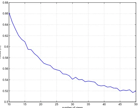
Subsection 3.3 considers the problem of directly estimating the transformation that maps from the Euclidian reconstruction coor-dinates to the georeferenced ones. To properly validate the pro-posed approach a Monte Carlo simulation (with 1000 indepen-dent samples) is considered: at each iteration of the Monte Carlo simulation a new set of values for the true camera positions and for the trueTg transformation are independently sampled. Then
the estimated device and optical center positions are assumed to be affected by zero-mean random Gaussian noises with standard deviations of 0.5 m and 0.02 m, respectively (accordingly with the assumption done in subsection 3.3 the variance of the error on the device positions is much larger than that of the error on the estimated optical centers). As shown in Fig. 5, the Root Mean Square Error (RMSE) of the estimated georeferenced device po-sitions with respect to their true values decreases following the expected1/√mbehavior (Anderson, 2003).
In our future work, we foresee a more in depth validation of the method by considering reconstructions on different real environ-ments, and the comparison with the results that can be obtained by means of bundle adjustment based reconstructions.
REFERENCES
Agarwal, S., Snavely, N., Seitz, S. and Szeliski, R., 2010. Bundle adjustment in the large. In: European Conference on Computer Vision, Lecture Notes in Computer Science, Vol. 6312, pp. 29– 42.
Anderson, T., 2003. An Introduction to Multivariate Statistical Analysis. John Wiley & Sons Inc., New York (U.S.A.).
10 15 20 25 30 35 40 45 50 0.5
0.52 0.54 0.56 0.58 0.6 0.62 0.64 0.66 0.68
number of views
RMSE (m)
Figure 5: Estimation error of the georeferenced positions (RMSE) varying the number of camera viewsm.
on Mobile computing and networking, MobiCom ’09, pp. 261– 272.
Bahl, P. and Padmanabhan, V., 2000. RADAR: An in-building RF-based user location and tracking system. In: IEEE INFO-COM, Vol. 2, pp. 775–784.
Brand, M., 2002. Incremental singular value decomposition of uncertain data with missing values. In: European Conference on Computer Vision, Lecture Notes in Computer Science, Vol. 2350, pp. 707–720.
Byr¨od, M. and Astr¨om, K., 2010. Conjugate gradient bundle ad-justment. In: European Conference on Computer Vision, Lecture Notes in Computer Science, Vol. 6312, pp. 114–127.
Cenedese, A., Ortolan, G. and Bertinato, M., 2010. Low-density wireless sensor networks for localization and tracking in criti-cal environments. Vehicular Technology, IEEE Transactions on 59(6), pp. 2951–2962.
Chiuso, A., Brockett, R. and Soatto, S., 2000. Optimal structure from motion: Local ambiguities and global estimates. Interna-tional Journal of Computer Vision 39(3), pp. 195–228.
El-Sheimy, N., Kai-wei, C. and Noureldin, A., 2006. The utiliza-tion of artificial neural networks for multisensor system integra-tion in navigaintegra-tion and posiintegra-tioning instruments. Instrumentaintegra-tion and Measurement, IEEE Transactions on 55(5), pp. 1606–1615.
Fischler, M. and Bolles, R., 1981. Random sample consensus: A paradigm for model fitting with applications to image analysis and automated cartography. Communications of the ACM 24(6), pp. 381–395.
Foxlin, E., 2005. Pedestrian tracking with shoe-mounted iner-tial sensors. Computer Graphics and Applications, IEEE 25(6), pp. 38–46.
Furukawa, Y., Curless, B., Seitz, S. and Szeliski, R., 2010. To-wards internet-scale multi-view stereo. In: Proceedings of the 23rd IEEE Conference on Computer Vision and Pattern Recogni-tion (CVPR), pp. 1434–1441.
Fusiello, A., 2000. Uncalibrated euclidean reconstruction: a re-view. Image and Vision Computing 18(6–7), pp. 555–563.
Goesele, M., Snavely, N., Curless, B., Hoppe, H. and Seitz, S., 2007. Multi-view stereo for community photo collections. In: Proceedings of the 11th IEEE International Conference on Com-puter Vision (ICCV).
Guarnieri, A., Pirotti, F. and Vettore, A., 2013. Low-cost mems sensors and vision system for motion and position estimation of a scooter. Sensors 13(2), pp. 1510–1522.
Hartley, R., 1997. In defense of the eight-point algorithm. IEEE Transaction on Pattern Recognition and Machine Intelligence 19(6), pp. 580–593.
Hartley, R. and Zisserman, A., 2003. Multiple View Geometry in Computer Vision. Cambridge University Press.
Heyden, A. and Astr¨om, K., 1996. Euclidean reconstruction from constant intrinsic parameters. In: Proceedings of the International Conference on Pattern Recognition, pp. 339–343.
Kennedy, R., Balzano, L., Wright, S. and Taylor, C., 2013. Online algorithms for factorization-based structure from motion. ArXiv p. 1309.6964.
Longuet-Higgins, H., 1981. A computer algorithm for recon-structing a scene from two projections. Nature 293(5828), pp. 133–135.
Lukianto, C. and Sternberg, H., 2011. Stepping – smartphone-based portable pedestrian indoor navigation. Archives of pho-togrammetry, cartography and remote sensing 22, pp. 311–323.
Ma, Y., Soatto, S., Koˇseck´a, J. and Sastry, S., 2003. An Invitation to 3D Vision. Springer.
Masiero, A. and Cenedese, A., 2013. Affinity-based distributed algorithm for 3d reconstruction in large scale visual sensor net-works. In: Proceedings of the 2014 American Control Confer-ence, ACC 2014, Portland, USA.
Masiero, A., Guarnieri, A., Vettore, A. and Pirotti, F., 2013. An indoor navigation approach for low-cost devices. In: Indoor Posi-tioning and Indoor Navigation (IPIN 2013), Montbeliard, France.
Morel, J. and Yu, G., 2009. ASIFT: A new framework for fully affine invariant image comparison. SIAM Journal on Imaging Sciences 2(2), pp. 438–469.
Piras, M., Marucco, G. and Charqane, K., 2010. Statistical anal-ysis of different low cost GPS receivers for indoor and outdoor positioning. In: IEEE Position Location and Navigation Sympo-sium (PLANS), MobiSys ’12, pp. 838–849.
Ruiz, A., Granja, F., Prieto Honorato, J. and Rosas, J., 2012. Accurate pedestrian indoor navigation by tightly coupling foot-mounted IMU and RFID measurements. Instrumentation and Measurement, IEEE Transactions on 61(1), pp. 178–189.
Snavely, N., Seitz, S. and Szeliski, R., 2008. Modeling the world from internet photo collections. International Journal of Com-puter Vision 80(2), pp. 189–210.
Tomasi, C. and Kanade, T., 1992. Share and motion from image streams under orthography: a factorization method. International Journal of Computer Vision 9(2), pp. 137–154.
Wang, H., Sen, S., Elgohary, A., Farid, M., Youssef, M. and Choudhury, R., 2012. No need to war-drive: unsupervised in-door localization. In: Proceedings of the 10th international con-ference on Mobile systems, applications, and services, MobiSys ’12, pp. 197–210.
Widyawan, Pirkl, G., Munaretto, D., Fischer, C., An, C., Lukow-icz, P., Klepal, M., Timm-Giel, A., Widmer, J., Pesch, D. and Gellersen, H., 2012. Virtual lifeline: Multimodal sensor data fu-sion for robust navigation in unknown environments. Pervasive and Mobile Computing 8(3), pp. 388–401.