Mutual fund evaluation: a portfolio insurance approach
A heuristic application in Spain
José M. Chamorro
a,∗, José M-
a. Pérez de Villarreal
b,1aDpt. Fundamentos del Análisis Económico, Instituto de Econom´ıa Pública, Fac. CC. Económicas y Empresariales, Univ. Basque Country,
Avda. Lehendakari Aguirre 83, 48015 Bilbao, Spain
bDpt. Econom´ıa, Fac. CC. Económicas y Empresariales (U. Cantabria), Avda. de los Castros s/n, 39005 Santander, Spain
Received 1 October 1998; received in revised form 1 August 1999; accepted 19 November 1999
Abstract
Usual techniques for evaluating mutual funds are based on asset pricing models (CAPM and APT) that are related to the mean–variance analysis, where risk aversion is assumed. Nonetheless we think that, at least in Spain and perhaps in continental Europe, a significant group of investors can be further portrayed by skewness preference. With this kind of investors in mind, we adopt a different approach based on option pricing theory. In particular, we show how to apply the portfolio insurance dynamics to the evaluation of mutual funds. We estimate insurance premia for 35 Spanish funds of diverse composition, and we also compute their net-of-downside-risk returns. We then rank funds according to both criteria. We also analyze the effect of transactions costs on these variables. © 2000 Elsevier Science B.V. All rights reserved.
JEL classification: G22; G12; D81
Keywords: Fund evaluation; Skewness preference; Portfolio insurance; Transactions costs
1. Introduction
Mutual funds are financial institutions that specialize in gathering family savings. The advantages they offer are well known. Savers can take part, through monetary contributions suitable for them, in financial asset portfolios managed by professionals who can diversify them in the right way, as they operate at great scale, incurring at the same time in low transactions costs. Thus, “market portfolios”, which enjoy efficient combinations of return and risk, become divisible and for the same reason accessible to less skilled savers. Besides, the liquidity of the shares is very high. Finally, favorable fiscal treatments also benefit participants. Due to all these advantages, it is not surprising that the savings gathered by funds in Spain be close to 33 billion Spanish pesetas by the end of 1998 (39% of GDP).
Not only have mutual funds multiplied their portfolio holdings but also their range has become wider. The offer is no longer limited to the traditional funds in monetary assets, fixed income assets with longer maturity,
∗Corresponding author. Tel.:+34-9460-13769.
E-mail addresses: [email protected] (J.M. Chamorro), [email protected] (J.M-a. P´erez de Villarreal).
1Tel.:
+34-9422-01649.
84 J.M. Chamorro,J.M-. P´erez de Villarreal / Insurance: Mathematics and Economics 27 (2000) 83–104
risky assets, and corresponding hybrids.2 The financial internationalization of the economy is mirrored in the appearance of funds with foreign asset portfolios as well as the increasing sensitivity of domestic portfolios to worldwide environment. Therefore, the crisis of international debt markets, which took place at the beginning of 1994, affected a great number of depositor-minded shareholders in Spanish funds. The feeling that taking part in mutual funds was not a decision without risk is what made them less attractive as a means of saving; the financial sector then reacted offering the so-called “guaranteed funds”.3 Financial upheavals during the sum-mer of 1997 and 1998 due to the worsening in Asian and Latin Asum-merican economies have surely reinforced this feeling.
More sophisticated funds will make rating more necessary. The protection of the less skilled savers also calls for an improvement in the information on the financial health of the funds. Though some funds be organized as “guaranteed”, there will be others (probably most of them) entailing risks. Taking part in the small and medium size firms, together with the opacity arising from operations with derivatives, will lead to shareholders undergoing a greater uncertainty. In this context, one might expect an increase in the demand for evaluation services.
The improvement in the “rating” activities favors low scale savers as it allows them to place their savings more efficiently. It also benefits the fund managers themselves as they are reported on their relative positions in a ranking of results. Finally, it also helps the supervising authorities to identify the most troublesome ones and to take action in safeguarding the interests of small scale investors.
The usual techniques for evaluating funds are based on asset pricing models (CAPM and APT) that are related to the mean–variance analysis, where risk aversion is assumed. In general, the use of these techniques is focused on equity or variable income funds. Besides, it is necessary to set a “benchmark portfolio” which in addition must be mean–variance efficient; otherwise the comparisons among different funds may be biased. Sharpe et al. (1995) provides a good overview of current practice in Chapter 25.
The starting point of this paper is that investors are further supposed to show strong skewness preference. We focus on those who are so sensitive to the risk of losing that they reject probabilistic distributions with negative skewness.4 In our opinion, there is a significant group of investors who can be portrayed in this way. Let us think, for example, about Spanish families and many others in continental Europe who have been traditionally savers rather than investors, most of whom have become new shareholders in the fund industry recently in spite of their depositor-minded profile. Perhaps by inertia, they are still used to safety, dreaming that “capital never vanishes”.
Skewness preference is in a sense similar to the asymmetrical risk perception behind the so-called “prospect theory” (Kahneman and Tversky, 1979; Tversky and Kahneman, 1992). They demonstrate that subjects’ choices of lotteries (or “prospects”) exhibit a wide range of anomalies that violate expected utility theory. In particu-lar, they show that losses loom much much larger than gains, an asymmetry of such magnitude that it can-not be explained by income effects or curvature in the classical utility function; they call this preference loss
2In Spain, fixed income funds (FIFs) are 100% composed of fixed income securities, mixed fixed income funds (MFIFs) are at least 75% fixed
income and at most 25% risky, mixed variable income funds (MVIFs) are at least 30% fixed income up to 75%, and variable income funds (VIFs) are more than 30% risky.
3At maturity, these funds reimburse as a minimum the initial capital plus a known rate and as a maximum the initial investment plus some
proportion of the gain in a stock index. The time to maturity is typically several years so they look like a term deposit; no surprise then that many investors disregard these products and turn to traditional funds.
4As is well known in the expected utility framework, risk aversion is characterized by the second derivative of the utility function(u′′(.) <0).
Skewness preference can also be considered by requiring the third derivative to be positive(u′′′(.) >0). To see it we simply apply Taylor’s expansion to the expected utility function:E[u(R)]=u(µ)+ 1
2!u′′(µ)σ 2
+ 1
3!u′′′(µ)κ+remainder, where E denotes expected value, R is the
portfolio return, andµ,σ2andκare the first three moments of its distribution. Now, providedu′′′(.) >0, the higher negative skewness the lower expected utility. Note that ifu′′′(.)takes a very high value then skewness effect may be strong enough to define a “loss rejection” behavior
aversion. Our loss rejection hypothesis could then also be interpreted as an extreme case of loss averse behavior.5
Although skewness preference can be accounted for in the expected utility context (see Footnote 4), the analysis becomes rather complex since we need to consider an additional parameter besides the usual mean and variance. On the other hand, “safety-first” models, which are also related to skewness preference while keeping mean–variance framework, deviate from the expected utility paradigm in a rather ad hoc way. This is why we propose a new approach to deal with “no-lose” investors.
The approach is based on option pricing theory. Particularly we focus on the “portfolio insurance” technique, and among others, we refer to previous important works such as those of Gatto et al. (1980), Leland (1980, 1985), Bookstaber and Clarke (1984), Rubinstein (1984), Benninga and Blume (1985), Benninga (1989), Bird et al. (1990) and Basak (1995).
We deem the portfolio insurance approach to be a quite natural way to grapple with the strong skewness prefer-ence.6 In short, the basic idea is as follows: if we purchase a stock and simultaneously purchase a put option on that stock, we know that the dollar return from the purchase will never be lower than the exercise price on the put. Let us now consider the possibility of insuring mutual funds in this way; then, for our investors, the best fund would be the one with the highest payoff provided they were insured against any potential loss, i.e., the one with the highest net-of-downside-risk return. In our case, there are not put options on the mutual funds in which we want to invest. However, under certain assumptions, their payoffs can be replicated by means of dynamic strategies involving the underlying portfolio and the riskless asset.
In this paper, we propose a measure of evaluation which is applicable, in principle, to all funds, either fixed or variable income funds. By making use of the portfolio insurance technique, we shall show how it is possible to build a ranking of funds according to their quality of risk and to their net-of-downside-risk return. Besides, it may be worth stressing that, concerning the information required, our method is hardly very demanding. We only take daily closing prices for each fund during the sample period together with the interest rate on the riskless asset. Given that a “benchmark portfolio” is not constructed, we are not able to spot which funds (if any) outperform the benchmark. In spite of this, performance is evaluated on a relative basis since we place the different mutual funds at the same starting point, at least to guarantee the investor’s initial wealth, and we rank them from best to worst according to the net-of-downside-risk (or hedged) returns they afford at the end of the investment period.
We show some results, such as the ranking by risk, which are not too surprising. Variable income funds are placed at the top positions, whereas fixed income ones are placed at the bottom. More surprises arise from the classifications by hedged return. There are equity funds which head the classifications and suggest that fixed or mixed fixed income are not always the most attractive shelter for those investors especially sensitive to the “risk of losing”. On the other hand, these rankings differ significantly from other more conventional ones based on raw return.
5Consider an investor with a utility function of the form:
a·RjifRj<0,
Rj ifRj≥0,
where Rjis the return on fund j, and a is a constant≥1. Such a function exhibits risk aversion in the large, because the loss in utility associated
with a return below zero is greater than the gain in utility associated with a return equally far above zero. Within return ranges that lie wholly above or wholly below zero, however, the function is linear and thus shows risk neutrality. The parameter a reflects the fact that, when considering the probability distribution of return, people weight possible losses more heavily than possible gains. A “no-lose” investor could then be described by an extremely high coefficient of loss aversion (a).
6Leland (1980) shows that investors who have average expectations on the return of the underlying stock, but whose risk tolerance increases
with wealth more rapidly than average, will wish to obtain portfolio insurance. Institutional investors falling in this class might include pension or endowment funds which at all costs must exceed a minimum value, but thereafter can accept reasonable risks. “Safety-first” investors would find portfolio insurance attractive on this basis. Note thatu′′′(.) >0 is a necessary condition to an increasing risk tolerance, as can be seen by differentiating the Arrow–Pratt measure of absolute risk aversionA= −u′′(.)/u′(.); so the link between skewness preference and portfolio
86 J.M. Chamorro,J.M-. P´erez de Villarreal / Insurance: Mathematics and Economics 27 (2000) 83–104
The paper is organized as follows: in Section 2, we explain the key theoretical elements of “portfolio insurance”; we then show how to work out indicators of risk and return, without and with (homogenous) transactions costs, that allow us to compare the different funds. In Section 3, we apply these measures to a heterogeneous group of 35 Spanish funds and build some classifications. We dedicate Section 4 to summarize the main results, make a wary comment, and suggest some further extensions. Finally, Appendix A reports some statistics concerning the goodness of the dynamic strategy as it impinges on our reliance on the results.
2. Portfolio insurance
There are n mutual funds in the market, the composition of which can be fixed income, variable income or mixed. Let Ftjbe the value in t of a share in fund j, where 0≤t≤1 andj =1, 2,. . ., n. We assume that the instantaneous
return on a share in a fund can be represented by the stochastic differential equation:
dFj
Fj =
µj·dt+σj·dZ, (1)
whereµj is the instantaneous expected return on the share in fund j,σj2the instantaneous variance of the return,
and dZ is an increment to a standard Gauss–Wiener process.
Initially we also assume “frictionless” markets: there are no transactions costs or differential taxes. Trading takes place continuously and borrowing and short-selling are allowed without restriction; investors can borrow and lend at the same rate.
2.1. Insurance premia as indicators of risk
Let us consider int =0 the possibility of investing A dollars in any one of these funds. We theoretically could aim at obtaining int =1 either a predetermined fraction of our initial wealth z·A if the fund goes wrong or the whole value of our investment in the fund if this performs nicely. In other words, we set a floor below which we do not want our wealth to fall while, at the same time, we do want to benefit from the upside return should there be any gain in the value of the share.
In this formulation z is a parameter that limits the chances of losing (z >0). The existence of a “free lunch” is not possible due to thez <er restriction, i.e., there is no way of insuring with certainty a greater return than a riskless asset, like a Treasury Bill. Ifz = 1, this structure of results would allow us to either benefit from any possible revaluation of the fund, or at least, to rescue the initial capital. We would be aiming at complementing our share in a fund with an insurance against losses. In the cases of values of z different from 1, this characteristic remains, though somehow qualified. The complementary insurance would obviously imply a cost.
It is well known that protecting oneself in this way is the same as buying put options on shares in the fund with maturity att =1 in a number wjand with an exercise price Kjsuch thatwjKj =z·A. In this context, an “insured
share” can be characterized as a compound asset involving a basic share and a put, the value of which would be the sumF0j +P0j(F0j, Kj), where P0j denotes the initial price of the derivative asset, which depends, among other
factors, on the value of the underlying asset and on the exercise price to be fixed.
Following Black and Scholes’ (B–S) option pricing model, the value of this compound asset would be
F0j+P0j(F0j, Kj)=F0j·N (hj)+Kj·e−r·N (σj−hj), (2)
where N(.) is the cumulative normal distribution function,hj ≡ln(F0j·er/Kj)/σj+σj/2, r the interest rate of a
riskless asset (Treasury Bills), andσjis standard deviation of the changes in the logarithm of the share price Ftj.
The number of insured shares that we could initially (t=0) buy with a sum of money A would be
The value wj determines the size of the global insured share, what we call “insured portfolio”. As stated previously,
in order to enjoy a perfect hedge, the minimum return insured by this portfolio must satisfy the equality
wjKj =z·A, (4)
from where the following expression is obtained
Kj
z =F0j·N (hj)+Kj·e
−r
·N (σj −hj). (5)
This is a nonlinear equation with only one unknown, Kj. Although it cannot be solved analytically, it is possible to
compute its solution by means of numeric procedures. Once Kj has been calculated, wj, P0j are determined, and
obviously, (F0j +P0j), which is the initial value of the synthetic asset or unitary insured share.
It should be noted that, from the start, we have been using hypothetical terms. The reason is that there are not any markets, at least for the time being, where call and put options on shares in funds are negotiated. Thus, the insurance price P0jis merely notional, and therefore cannot be observed. Nevertheless, it can be computed, and we deem this
exercise to be useful from an informative point of view.
The information embedded in them would allow us to give an answer to questions such as how much the fund managers ought to pay an insurance company should they want to insure shareholders’ contributions. The fact that this kind of insurance is not traded does not invalidate the informative function of P0j. These prices, though merely
notional, are still a monetary evaluation of the risk of losing in a fund. For the same reason, they are useful to us as a criterion for establishing a ranking based on risk. Thus, int =0, fund j is perceived as involving a higher risk than fund h if(P0j/F0j) > (P0h/F0h). The idea is very clear: notionally more expensive insurance reveals greater
latent risks.
2.2. Risk-adjusted returns as indicators of performance
Needless to argue that investors are concerned with both risk and return. Financial theory focuses on risk measuring and pricing, while risk-adjusted return (RAR) is assumed to be the ultimate objective investors pursue to maximize. Whatever the criterion considered to deal with risk, the basic idea remains the same, namely that raw return must be adjusted for or discounted by risk. In the CAPM framework, for instance, RAR is formulated as the mean return minusβtimes the excess market return,β being the risk parameter.
In our case of no-lose investors, a naive way to introduce the notion of downside-risk-adjusted return (DRAR) would be as follows:
DRARj =
Rj− P0j/F0j·er if Rj >0,
− P0j/F0j·er if Rj ≤0,
where Rj is the raw return on fund j at the end of the investment period (t =1), and (P0j/F0j) er appraises the risk
of losing. It can be seen that DRARjhas a floor, but no ceiling. In fact, this is the return on an insured portfolio, i.e.,
a portfolio made from basic shares and put options att =0 so that investors could take no risk of losing. Clearly, DRARjis an adjusted return since it is net of the payment for protection (P0j/F0j) er. Note, though, that DRARj
has a serious drawback, as it is deeply related to the last day of the period; this suggests that some sort of average value ought to be used in order to evaluate funds comparatively.
88 J.M. Chamorro,J.M-. P´erez de Villarreal / Insurance: Mathematics and Economics 27 (2000) 83–104
With the passage of time and as the involved variables change in value, these weights must be readjusted. Having reachedt=1, this portfolio, with its final composition, will have a certain value CV1jwhich will define, in relation
to the initial wealth A, a rate of returnRcj=(CV1j−A)/Awhich we shall call covered (or hedged) return.
Analogously to DRARj, Rcj is the rate of return on an insured share in fund j (i.e., insured against the risk of
losing). We are therefore also dealing with a net-of-downside-risk return. However we think Rcj is a more precise
indicator than DRARj, since it evolves continuously through the whole investment period. Although it is more
complex to calculate, we opt to rely on Rcj for the sake of accuracy.
As we are thinking about “no-lose” investors, Rcj is supposed to be the key return in order to compare different
funds. So we claim that fund j is better ranked than fund h ifRcj > Rchin a given period. To be sure: we place the different mutual funds in the same starting point (at least to guarantee the initial capital A) and we rank them from best to worst according to the net-of-downside-risk returns they afford at the end of the investment period (in t =1). Concerning its empirical implementation below, since we analyze 16 quarterly periods, it seems convenient to look at some average measure of these quarterly values. As we argue later on, the geometric mean fits reasonably well in this loss aversion context.
2.3. Introduction of transactions costs
Up to now, we have not taken into account the transactions costs in the P0jand Rcjformulations. It is nevertheless
clear that these do exist and that they affect, to a greater or less extent, the dynamic management required to replicate the “insured portfolio”. Following Leland (1985) we can distinguish two effects derived from these costs:
(1) A “transactional frequency” effect takes place. Logically, if there are costs, the trade in assets diminishes. Because of this, the dynamism of portfolio revision slows down and the hedge or replication of the synthetic portfolio turns out more imperfect.
(2) The “volatility” effect is the other and can be put in the following way:
ˆ
where 2c is the cost of a round trip transaction (purchase and sale, or the other way round),σˆ2the variance with costs, andσ2is the variance without costs. The idea underlying this formula is that transactions costs drive a wedge between the effective closing prices of mutual funds.
The introduction of transactions costs leads to a rising revision of the P0jinsurance costs due to greater volatility,
and in general, it tends to reduce the return on the replicating portfolio Rcj.
We shall now proceed to look over the arithmetics of the model when transactions costs are incorporated. Letαtj be the percentage of A to be invested in fund j at date t. Obviously, the existence of costs implies that a different percentageβtjought to be purchased. The revision of the model basically consists in defining the relation between
αtj andβtj.
For this, let us once again place ourselves int =0. If an order to acquire a percentageβ0j of shares is placed,
a cost will have to be paid on the difference between the acquired percentage and that of the start (which is zero), that is, c timesδ0j, whereδ0j =β0j−0.
The initial net wealth (after having placed the order) will be
that is, the sum of the quantities invested in the fund and in the riskless asset. Note that (β0j−c·δ0j) is a fraction,
asδ0j =β0j, and for the same reason,(β0j−c·δ0j)=β0j·(1−c).
Ifα0jis the desired investment, then the following ought to take place
α0j =
Up to now we have referred to the initial moment. In order to consider dates within the investment period which we have normalized to be 0≤t≤1, let us agree on dividing this in n days and on using the subindexτ =1, 2,. . ., n to date the variables on a daily basis. Let us also assume that after one more day (τ =1) the fund has grown by a factor of x1, and the riskless asset according to er·1t. The wealth at the beginning of the following day would be
A·[α0j·x1+(1−α0j)·er·1t]·(1−c·δ0j)≡A1. (11) With this new initial wealth and the current price of the share, the corresponding proportionα1jis determined. Be
β1j the new purchase order under transaction costs; we then have
δ1j ≡
Previously to the analysis of the results obtained, certain characteristics of the data used ought to be commented upon.
3.1. Data
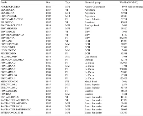
90 J.M. Chamorro,J.M-. P´erez de Villarreal / Insurance: Mathematics and Economics 27 (2000) 83–104 Table 1
Some characteristics of the funds in the sample
Funds Year Type Financial group Wealth (30-VI-95)
AHORROFONDO 1986 MFI Ahorro Corporaci´on 5975 million pesetas
BEX BOLSA 1987 VI Argentaria 4371
SUPERFONDO ST II 1986 MFI Banco Santander 109369
As there is certain freedom of composition, some of the funds have changed category, going from one modality to another, during the sample period.
The aggregate wealth of the funds in the sample is quite significant, having doubled during the period under con-sideration (from 955 044 million Spanish pesetas at the end of 1991 up to 1 886 275 million by mid 1995). In 1995 it represented about 40% of the patrimonial value of the whole of the funds. On the other hand, the distribution accord-ing to types is biased towards fixed income, which represents 67% of the aggregate wealth, whereas variable income hardly surpasses 4%. The rest is all in mixed income, although in these funds fixed income securities also prevail.
Most of the funds analyzed are managed by a few companies linked to bank groups (the numbers in brackets refer to year 1995): Banco de Santander (6 and 14.8% of aggregate wealth), La Caixa (6 and 36.3%), Banco Central Hispano (5 and 8%), Banco Bilbao Vizcaya (4 and 20%), Argentaria (3 and 7.25%), Banco Popular (2 and 3%), and Banesto (2 and 2.8%). This concentration would allow us to study both risk and performance behaviors by bank groups.
Transforming the closing prices of the different funds into daily logarithmic returns has been a first treatment of data series. Afterwards their quarterly standard deviations have been calculated so as to use them as measures of volatility in the B–S formula. In particular,σj has been estimated from daily returns for the concerned quarter.7
Finally, the quarterly interest rates of the riskless asset are those of the Treasury Bills (TB).
3.2. Results
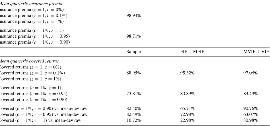
First, we look at the insurance premia estimated as indicators of funds’ risk; then we put some emphasis on the “covered” or hedged returns and compare them with the raw returns on funds. In both parts, we carry out a sensitivity analysis towards transactions costs and rescue thresholds assuming three different levels for c (0, 0.1 and 1%) and z (0.90, 0.95, and 1). Nevertheless, the pair of values (c=1%,z=1) stands as the base case, since we think they reflect more accurately the actual costs8 and the strong loss aversion hypothesis.
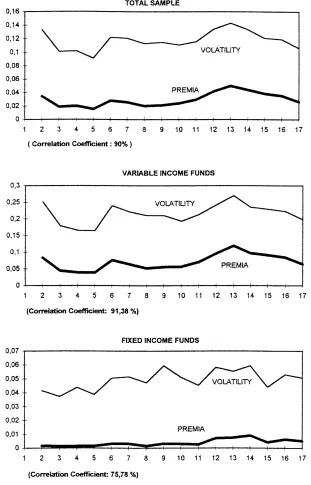
As it is shown in Figs. 1 and 2 below, both insurance premia and covered returns vary throughout the 16 quarterly periods so any ranking based on the last estimates may seem rather myopic. In consequence, we deem it sensible to rely on some average values in order to rank the funds more consistently. For this purpose we apply the arithmetic mean to the premia estimates whereas we use the geometric mean in the case of the covered returns. This is computed here as
We propose the geometric mean of the RARs as a global indicator of performance since it sounds well in a loss aversion context. This measure penalizes extreme values, specially the negative ones. In fact, a portfolio with any ruinous event would have a zero geometric mean and consequently would be ranked in the last position. In
other words, note that both(1+RGcj)and ln(1+RGcj)lead to the same ranking since the latter is a monothonic transformation of the former, and that ln(1+RcGj)= 161 P16
i=1ln(1+Rcij). According to the right-hand side, it is
easily shown that the negative values of Rcare more and more weighted than the positive ones.9 Note that covered
7We thus measure historical risk and performance, which are not necessarily indicative about future. Historical results are nonetheless useful
and interesting information. Before deciding how to invest going forward, investors are likely to want to know how various funds performed in the past, and whether they were adequately compensated for the risks they faced.
8Keep in mind that it is 1% due both to an entry operation (purchase of shares in the fund) as well as an exit operation (sale). Therefore, we are
not dealing only with a standard refunding fee but, in these costs, mutual fund entry charges are also included. For example, if the adjustment in the replicating portfolio involved selling today the same sum that it is to be purchased tomorrow, the transaction cost incurred would be 2% of such sum. Capital gains or losses implied by these readjustments are taxable but we do not analyze this effect.
9As discussed in Footnote 5, it is possible to represent the intuition of a no-lose behavior in a utility/return space by means of a kink in the
92 J.M. Chamorro,J.M-. P´erez de Villarreal / Insurance: Mathematics and Economics 27 (2000) 83–104
94 J.M. Chamorro,J.M-. P´erez de Villarreal / Insurance: Mathematics and Economics 27 (2000) 83–104
returns can be negative because of imperfect or incomplete hedging (due both to discontinuous trading, transactions costs and/or rescue values below unity).
Thus, and for the sake of briefness, we only present the average estimates of the both variables we have just mentioned. They are shown at individual level so as to outline classifications according to risk and return, as well as at group level (FI, MFI, MVI, VI and total of the sample) so as to make comparisons among the different types of funds.
3.2.1. Insurance premia and classifications by risk
As explained above, Eq. (5) of the previous section can be solved for one unknown, Kj, by a numerical routine10
for each observed F0j and σj; when transactions costs are considered, the standard deviation is transformed
according to Eq. (7). Then, given the solution value (Kj), an estimate of the insurance premium P0jcan be computed
using Eq. (2) and hence the ratio P0j/F0j.
We have followed this procedure for each of the sample funds on a quarterly basis over the study period (16 quarters, from 1 July 1991 until 30 June 1995) with the different transaction costs (0, 0.1, and 1%) and threshold values (0.90, 0.95, and 1). We set the time to expiration at 0.25, implicitly assuming that, in purchasing insurance, funds buy a net put every quarter with a maturity of 1/4 year.
Aggregate results. Fig. 1 shows the time evolution of the insurance premia of the whole sample, as well as the specific ones of the VIFs and FIFs, computed under the base assumptions ofc=1% andz=1. Note the great correlation between premia and volatility in the case of VIFs, and also in all of the sample; not so in the FIFs group, where the size of both variables is significantly more reduced. On the graphs (mainly in the variable income one) it is the peaks of the quarterly periods of July–September 1992, and April–June 1994, that stand out, periods during which financial markets run into trouble. The relatively high premia of VIFs are also explained by the increase in volatility derived from transactions costs.
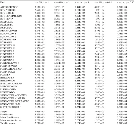
All the aggregate results are shown, by means of simple averages, at the bottom of Table 3. We can here observe that the whole average premium is 7.62‰if at least a 100% of the initial investment is guaranteed and no transaction costs are considered. Nevertheless, in the case of including these costs (0.1 and 1%), premia increase at 9.89‰and at 2.94%, respectively. Thus we are aware that insurance premia are effectively sensitive to transactions costs. At greater cost there is more volatility, and for the same reason the price of the insurance increases.
The same sensitivity is observed between insurance premia and rescue levels. Focusing on the casec=1%, the results show that the higher the values of z demanded, i.e., 0.90, 0.95 and 1, the greater the premia required, 2.40‰ 7.65‰and 2.94%.
As expected, the price of the insurance differs significantly among the different types of funds. From 7.03% (with c=1%), as an average of the 16 quarters, in those of variable income, to much lower levels, about 3.77‰, in those of fixed income. Therefore, the figures are consistent with the supposition that funds involving higher risks ought to pay more for insuring their wealth. Note that this relation takes place for the different values of c and z.
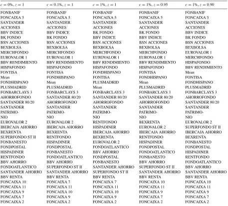
Individualized results and classifications. Table 3 also details our individualized calculations under the different assumptions about transactions costs and rescue levels. The central column remakes the base case (c=1%,z=1). On the other hand, Table 4 displays the five classifications of funds based on these figures. The ranking is from greater to less risk (as gauged by premium). This table worths more commenting.
First, as it is logical, FIFs appear at the lowest positions, whereas VIFs are at the head of the ranking. Among these, FONBANIF has the first position with 8.83%. On the other hand, among those of fixed income, there are funds (FONCAIXA, mainly) with very small premia. In general, FIFs are positioned behind MFIFs, these follow MVIFs, which, in turn, appear behind VIFs. Nevertheless, FONCAIXA 5 (especially) and EUROVALOR 1, both in the MVI segment, appear as involving higher risk than some of VI.
10We used subroutine BRENTM (algorithm no. 504, ACM). In a trial run, we found that the convergence is not sensitive to the initial estimates of
the solution. The initial estimate that we used for the value, Kj, was the actual price at the beginning of the investment period, that is, the closing
Table 3
Quarterly Insurance Premia (period: July 1991 to June 1995)
Fund c=0%,z=1 c=01%,z=1 c=1%,z=1 c=1%,z=0.95 c=1%,z=0.90
Second, the classifications hardly differ due to the transaction costs and the rescue thresholds. As it is summarized in Table 7, Kendall’s concordance coefficient11 among rankings withc=0, 0.1 and 1% under the assumptionz=1 (the first three columns in Table 4) is 98.94%, which suggests the classifications are not sensitive to homogeneous costs. On the other hand, a similar result is obtained when the comparison is made among rankings withz=0.90, 0.95 and 1 underc=1% (the last three columns), since correlation also approaches 99%.
11Kendall (1963, Chapter 6) defines the coefficient of concordanceW
=(12·S)/m2·(n3−n), where m is the number of rankings, n is the number of funds, and S is the sum of squares of the actual deviations between the sum of ranks for each fund and the mean value of the sums,
1
96 J.M. Chamorro,J.M-. P´erez de Villarreal / Insurance: Mathematics and Economics 27 (2000) 83–104 Table 4
Rankings by mean insurance premia (period: July 1991 to June 1995)
c=0%,z=1 c=0.1%,z=1 c=1%,z=1 c=1%,z=0.95 c=1%,z=0.90
FONBANIF FONBANIF FONBANIF FONBANIF FONBANIF
FONCAIXA 5 FONCAIXA 5 FONCAIXA 5 FONCAIXA 5 FONCAIXA 5
SANTANDER
BBV INDICE BBV INDICE BK FONDO BK FONDO BBV INDICE
BK FONDO BK FONDO BBV INDICE BBV INDICE BK FONDO
BSN ACCIONES BSN ACCIONES BSN ACCIONES BSN ACCIONES BSN ACCIONES
BEXBOLSA BEXBOLSA BEXBOLSA BEXBOLSA BEXBOLSA
MERCHFONDO MERCHFONDO MERCHFONDO MERCHFONDO EUROVALOR 1
EUROVALOR 1 EUROVALOR 1 EUROVALOR 1 EUROVALOR 1 MERCHFONDO
BBV RENDIMIENTO BBV RENDIMIENTO BBV RENDIMIENTO BBV RENDIMIENTO HISPAFONDO
HISPAFONDO HISPAFONDO HISPAFONDO HISPAFONDO BBV RENDIMIENTO
FONTISA FONTISA FONDHISPANO FONTISA Mean
Mean FONDHISPANO FONTISA FONDHISPANO FONTISA
FONDHISPANO Mean PLUSMADRID Mean FONDHISPANO
PLUSMADRID PLUSMADRID Mean PLUSMADRID PLUSMADRID
FONBARCLAYS 3 FONBARCLAYS 3 FONBARCLAYS 3 FONBARCLAYS 3 FONBARCLAYS 3
AHORROFONDO SANTANDER 80/20 SANTANDER 80/20 SANTANDER 80/20 AHORROFONDO
SANTANDER 80/20 AHORROFONDO AHORROFONDO AHORROFONDO SANTANDER 80/20
EUROVALOR 2 EUROVALOR 2 RENTFONDO BEXRENTA EUROVALOR 2
IBERCAJA AHORRO IBERCAJA AHORRO HISPADINER EUROVALOR 2 SUPERFONDO ST II
BEXRENTA BEXRENTA IBERCAJA AHORRO IBERCAJA AHORRO IBERCAJA AHORRO
SUPERFONDO ST II RENTFONDO BEXRENTA RENTFONDO BEXRENTA
FONBANESTO HISPADINER EUROVALOR 2 HISPADINER FONBANESTO
FONDPOSTAL FONDPOSTAL FONDOATLANTICO FONDPOSTAL FONDPOSTAL
HISPADINER FONBANESTO BBV AHORRO FONDOATLANTICO HISPADINER
RENTFONDO FONDOATLANTICO FONDPOSTAL FONBANESTO RENTFONDO
BBV AHORRO BBV AHORRO FONBANESTO BBV AHORRO FONDOATLANTICO
FONDOATLANTICO SUPERFONDO ST II SANTANDER AHORRO SUPERFONDO ST II BBV AHORRO SANTANDER AHORRO SANTANDER AHORRO SUPERFONDO ST II SANTANDER AHORRO SANTANDER AHORRO
BBV RENTA BBV RENTA BBV RENTA BBV RENTA BBV RENTA
FONCAIXA 10 FONCAIXA 7 FONCAIXA 7 FONCAIXA 10 FONCAIXA 10
FONCAIXA 11 FONCAIXA 11 FONCAIXA 11 FONCAIXA 11 FONCAIXA 11
FONCAIXA 9 FONCAIXA 10 FONCAIXA 10 FONCAIXA 9 FONCAIXA 9
FONCAIXA 7 FONCAIXA 9 FONCAIXA 9 FONCAIXA 7 FONCAIXA 7
FONCAIXA 2 FONCAIXA 2 FONCAIXA 2 FONCAIXA 2 FONCAIXA 2
3.2.2. Covered returns and corresponding classifications
In the previous section we have estimated the insurance premium for each fund on each quarterly period. It is then straightforward to compute the initial proportions of the underlying asset and the riskless asset in the replicating portfolio by means of Eq. (6). Henceforth the pattern of readjustments goes along the lines described by Eqs. (8)–(15) with c adopting the value stated in each case.
We follow the same order of presentation as before. We only add a section where classifications of funds according to “covered” or hedged returns are compared to other more traditional ones based on raw returns.
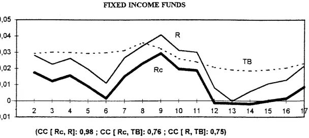
the profiles of their returns are compared with the return on a substitute asset, the Madrid Stock Exchange General Index (IGBM) in the case of variable income, and TB in that of fixed income.
Note that the covered return does not significantly go into the area of negative values, as is logical, whereas the raw return and that of the IGBM do. The value of Rcapproaches zero in the quaterly periods in which the financial markets plummet. On the other hand, this return, not because of being insured, is fixed or invariant; in fact, it varies more than the return on TB. The latter dominates (evolves above) Rc, but not so the raw return. Finally, the global correlation between Rcand R is 93%, 91% in the case of VIFs and 98% in that of FIFs. From Fig. 1 it is also very easy to test that the quarterly frequency distribution does not show negative skewness in the Rccase while it is much more symmetrical when R is considered. The former is just the profile which would logically be appreciated by investors with strong skewness preference.
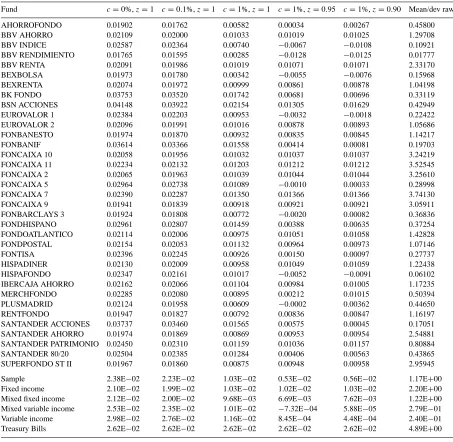
Table 5 at the bottom collects our estimates of Rcjfor 16 quarters, both at the aggregate and segment level, under
the different costs and thresholds considered. As can be seen, there are no surprises in the relation between return and transaction costs: the quarterly covered return is reduced as costs are greater. This reduction affects especially VIFs and MVIFs which, due to their composition, are more exposed to the portfolio dynamic revision, though they are not clearly dominated by FIFs nor MFIFs.
The relation between return and rescue value is less clear. For each set of funds, the mean covered return increases as the threshold increases from z = 0.90 to z = 1, but except for VIFs it decreases at z = 0.95. The setting of a floor becomes particularly convenient when a loss takes place; otherwise it represents just a sunk, worth avoiding cost. Although not reported here,12 it is possible to show that whenever a fund loses more than 5% on some period (so that the rescue requirement turns binding), the inequalityRicj (z =0.95) > Rcij (z = 0.90) holds; it can then be said that the “threshold-effect” more than offsets the “premium-effect”. Conversely, when the fund’s loss is less significant the latter dominates the former andRcij (z = 0.90) > Ricj (z=0.95).
Most of the losses, both in frequency and size, refer to the MVI and VI segments, especially to the latter. Concerning VIFs, the number of losses is almost evenly distributed above and below 5% so on average it is possible to observe that the higher the value of the floor, the higher the covered return. However, only one in three of the losses in the MVIFs is greater than 5%; the relation between z and Rcis thus blurred since the a priori riskier strategy (z =0.90) is cheaper than the more conservative one (z =0.95). In other words, as the chance of a heavy loss decreases the premium-effect overshadows the threshold’s role. The same fact may be operating in the MFI and FI segments (Rcdecreases as z increases from 0.90 to 0.95) though less strongly since their insurance premia are noticeably lower.
Finally, the interest rates of TB almost always surpass the average covered returns on funds, with few exceptions (variable income with low costs); look at the bottom line in Table 5. As TB also lack the risk of losing, even investors with strong skewness preference should have preferred them to insured funds. How can then be explained that they invested in funds? First of all, shall we clear it, return dominance of the TB and other riskless assets was really evident in the fact that the greatest slice of household savings had flowed to them over the years 1991–1995; only 5200 billion pesetas (less than 5% of households and non-financial firms assets) were poured in funds by the end of 1995. Note further that, as mentioned before, fixed income funds represented about two thirds of that figure. On the other hand, fiscal advantages, and perhaps investments by people less sensitive to risk, can explain this remainder of wealth placed in funds. In any case, we think that the return dominance of TB has been vanishing along with the fall in interest rates during the last years.
Individualized results and classifications. Once again we are more interested in the ranking than in remarking the quantitative individualized estimates reported in Table 5. The only one detail we insist on is the negative values of the geometric mean returns that emerge for some funds when the rescue threshold is lower than unity. There are
12The reader interested in these results or in the individualized estimates of premia and returns under the different assumptions and periods can
98 J.M. Chamorro,J.M-. P´erez de Villarreal / Insurance: Mathematics and Economics 27 (2000) 83–104 Table 5
Quarterly covered and raw returns (period: July 1991 to June 1995)
Fund c=0%,z=1 c=0.1%,z=1 c=1%,z=1 c=1%,z=0.95 c=1%,z=0.90 Mean/dev raw
AHORROFONDO 0.01902 0.01762 0.00582 0.00034 0.00267 0.45800
BBV AHORRO 0.02109 0.02000 0.01033 0.01019 0.01025 1.29708
BBV INDICE 0.02587 0.02364 0.00740 −0.0067 −0.0108 0.10921
BBV RENDIMIENTO 0.01765 0.01595 0.00285 −0.0128 −0.0125 0.01777
BBV RENTA 0.02091 0.01986 0.01019 0.01071 0.01071 2.33170
BEXBOLSA 0.01973 0.01780 0.00342 −0.0055 −0.0076 0.15968
BEXRENTA 0.02074 0.01972 0.00999 0.00861 0.00878 1.04198
BK FONDO 0.03753 0.03520 0.01742 0.00681 0.00696 0.33119
BSN ACCIONES 0.04148 0.03922 0.02154 0.01305 0.01629 0.42949
EUROVALOR 1 0.02384 0.02203 0.00953 −0.0032 −0.0018 0.22422
EUROVALOR 2 0.02096 0.01991 0.01016 0.00878 0.00893 1.05686
FONBANESTO 0.01974 0.01870 0.00932 0.00835 0.00845 1.14217
FONBANIF 0.03614 0.03366 0.01558 0.00414 0.00081 0.19703
FONCAIXA 10 0.02058 0.01956 0.01032 0.01037 0.01037 3.24219
FONCAIXA 11 0.02234 0.02132 0.01203 0.01212 0.01212 3.52545
FONCAIXA 2 0.02065 0.01963 0.01039 0.01044 0.01044 3.25610
FONCAIXA 5 0.02964 0.02738 0.01089 −0.0010 0.00033 0.28998
FONCAIXA 7 0.02390 0.02287 0.01350 0.01366 0.01366 3.74130
FONCAIXA 9 0.01941 0.01839 0.00918 0.00921 0.00921 3.05911
FONBARCLAYS 3 0.01924 0.01808 0.00772 −0.0020 0.00082 0.36836
FONDHISPANO 0.02961 0.02807 0.01459 0.00388 0.00635 0.37254
FONDOATLANTICO 0.02114 0.02006 0.00975 0.01051 0.01058 1.42828
FONDPOSTAL 0.02154 0.02053 0.01132 0.00964 0.00973 1.07146
FONTISA 0.02396 0.02245 0.00926 0.00150 0.00097 0.27737
HISPADINER 0.02130 0.02009 0.00958 0.01049 0.01059 1.22438
HISPAFONDO 0.02347 0.02161 0.01017 −0.0052 −0.0091 0.06102
IBERCAJA AHORRO 0.02162 0.02066 0.01104 0.00984 0.01005 1.17235
MERCHFONDO 0.02285 0.02080 0.00895 0.00212 0.01015 0.50394
PLUSMADRID 0.02124 0.01958 0.00609 −0.0002 0.00362 0.44650
RENTFONDO 0.01947 0.01827 0.00792 0.00836 0.00847 1.16197
SANTANDER ACCIONES 0.03737 0.03460 0.01565 0.00575 0.00045 0.17051
SANTANDER AHORRO 0.01974 0.01869 0.00869 0.00953 0.00954 2.54881
SANTANDER PATRIMONIO 0.02450 0.02310 0.01159 0.01036 0.01157 0.80884
SANTANDER 80/20 0.02504 0.02385 0.01284 0.00406 0.00563 0.43865
SUPERFONDO ST II 0.01967 0.01860 0.00875 0.00948 0.00958 2.95945
Sample 2.38E−02 2.23E−02 1.03E−02 0.53E−02 0.56E−02 1.17E+00 VIFs so the above discussion about premium- and threshold-effect probably applies.
100 J.M. Chamorro,J.M-. P´erez de Villarreal / Insurance: Mathematics and Economics 27 (2000) 83–104
Secondly, we look at the base case (z = 1, c = 1%) in order to remark the feature ranking. Unlike the one based on insurance premia, this is no longer a staggered juxtaposition or the different partial, or by seg-ments, classifications we could consider. All of them appear rather mixed. So there are some VIFs and MV-IFs at the top (BSN ACCIONES, BK FONDO, SANTANDER ACCIONES, FONBANIF, FONDHISPANO) and others at the bottom (BBV RENDIMIENTO, BEXBOLSA, PLUSMADRID, BBV INDICE). The same is ob-served amongst the FIFs or MFIFs (RENTFONDO, FONDBARCLAYS 3, AHORROFONDO are at lower posi-tions, but FONCAIXA 7, FONCAIXA 11, SANTANDER 80/20 and SANTANDER PATRIMONIO are at higher ones).
It is worth recalling that two elements have an influence on Rcj: the revaluation of the fund and the risk of losing.
Both factors explain the good behavior of fixed income. Not only does it involve less risk (the discount is very small) but the base return was substantial.
It seems that in some funds the risk discount has contributed to their low covered returns; for example, the two that head the ranking by risk (FONBANIF and FONCAIXA 5) do not head the classification by return. Nevertheless, it seems that the last positions of others, like BEXBOLSA and BBV RENDIMIENTO, cannot be explained exactly due to their degree of risk but to their poor revaluation. Conversely, the positions held by some of VIFs (BSN ACCIONES, BK FONDO) seem to obey to their great revaluation and not to their low discount for risk, as their insurance premia are substantial and their position in the ranking by risks relatively high.
The fact that several VIFs appear in the highest part of the ranking shows that not always those of FI, let alone those of MFI, are the ones that offer higher insured return. In this case, even wise investors, whose preferences aim at “not to lose”, should find them attractive.
Finally, following our calculations it is also possible to outline, although not clearly enough, a ranking by bank groups. In this sense, it seems that the one led by Banco de Santander (because of its funds in VI and MFI) is at the top, and that of BBV at the bottom (mainly because of its VIFs); La Caixa would be in the middle of the ranking.
Comparing these classifications to the other ones, particularly the referred to the base case (c = 1%,z =1), some great differences can be observed. In fact Spearman’s correlation coefficient13 amounts to 10.72% when all the funds are accountd for (23% in the case of fixed income and 31% in variable income).
As it is collected in Table 7, the correlation is much higher when lower values for z are considered. In particular for variable income funds, as the size of the allowable loss increases the value of the Spearman’s coefficient also increases (reaching 90.76% whenz=0.90).
4. Summary, cautions and extensions
In this work we have shown how to apply the “portfolio insurance” theory to the evaluation of mutual funds. In particular, we have estimated the insurance premia for 35 Spanish funds of diverse composition, and we have also computed their net-of-risk-of-losing returns. Following these calculations we have made classifications based on their risk and hedged return.
There are some results, such as the ranking by risk, which are not too surprising. Variable income funds are placed in the first positions, whereas fixed income ones are placed in the last. This ranking is quite robust when faced with changes in the (homogeneous) transaction costs and the rescue values, as is shown in Table 7 where Kendall’s correlation coefficients display high values.
More surprises arise from the classifications by “covered” return. There are variable income funds which head the classifications and suggest that fixed or mixed fixed income are not always the most attractive shelter for those investors especially sensitive to the “risk of losing”. Our relative evaluations of funds turn out to change slightly when transactions costs are considered, but a bit more with the rescue thresholds. On the other hand, these classifications differ significantly from other more conventional ones based on the raw return.
Using again the Kendall indicator, we can conclude that the differences in ranking due to the transactions costs amount to 11%, while they get to 26% with respect to rescue values. Besides, the divergence between our ranking and the more conventional one gets to 89%. Obviously, some remarkable individual differences are also appreciated.
At this point, we cannot help warning about the confidence we should put in these results. As we briefly argue in Appendix A, the dynamic hedging strategy we have used to compute risk premiums and covered returns is certainly faulty. About half the days the replicating portfolio does not fulfill its purpose, i.e., it falls below the floor. However, the gaps do not seem to be so significant as to jeopardize our analysis especially when it concerns to rankings, since their size is nearly the same amongst funds.
This work can be qualified and extended in several ways. It could be assumed, for example, a lower frequency of transactions (weekly, not daily, revision of the replicating portfolio or, alternatively, conditioned to the fact that the fluctuations of the closing value surpass certain levels). The results can also be qualified taking into consideration other measures of the volatility of the funds’ return (for example, on the basis of the data of the previous quarterly period, and not of the quarterly investment horizon itself).
A more challenging extension would account for heterogeneous transaction costs. It has been assumed in this work that they are the same for the different mutual funds. It would be interesting to consider heterogeneous levels (percentages) of such costs, although the information required for this does not seem to be easy to obtain.
Another substantial improvement would be to relax, partially or totally, the assumption of constant volatility of the B–S model. Obviously, the calculations of the costs of the insurance and of the hedged return become much more complex, but any effort aiming at this goal would be worthwhile. In this sense, the possibility of introducing volatility estimates based on ARCH models can be looked into.
13The Spearman rank correlation coefficient is defined asr
=1− 6Pni=1di2/(n3−n)
, where n stands for the number of funds, and didenotes
102 J.M. Chamorro,J.M-. P´erez de Villarreal / Insurance: Mathematics and Economics 27 (2000) 83–104
Acknowledgements
We kindly thank the Comisión Nacional del Mercado de Valores (CNMV), and especially D¯a. Nieves Garc´ıa Santos, for providing the data used in this research. We also acknowledge the seminar participants at the University of the Basque Country, European University of Madrid, and the participants at the European Institute for Advanced Studies in Management (Brussels), and the French Finance Association Annual Meeting (Lille). We particularly thank an anonimous referee for his/her comments on an earlier version of this paper. J.M.C. also acknowledges financial support from the Ministerio de Educación y Ciencia (MEG PB96-1469-C05-02). The co-authors are responsible for any remaining errors.
Appendix A. On the shortcomings of dynamic hedging strategy
The dynamic strategy we implement in this paper must be taken warily on several grounds. First, the process governing the return on each fund may not be as simple as the one assumed in our framework (Eq. (1)).
Second, the model assumes that portfolio weights are continuously adjusted, whereas we have waited a whole day to readjust our proportions; moreover, since readjustment of the portfolio involves transactions costs to the investor, only finite adjustment is possible.
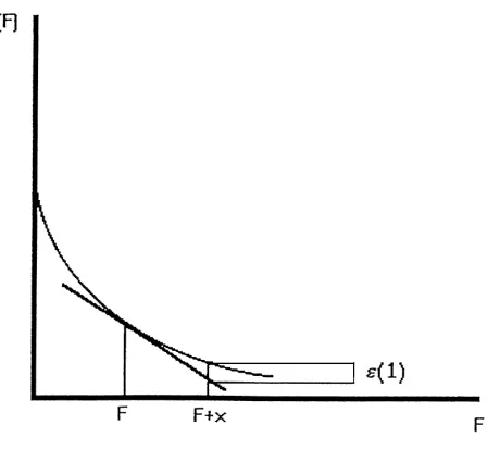
The third trouble requires a rather more technical explanation. For small changes in the underlying price, we know from calculus that a reasonably accurate measure of the change in market value of a put’s price is obtained from the usual first-order approximation:
Pj(Fj+x)=Pj(Fj)+P′j(Fj)·x+ε(1) (A.1)
where Pj(Fj) is the price of a put at a particular time and at a price level Fj for the underlying, the delta (1) of
the derivative is the slopeP′j(Fj)of the graph of P at F, andε(1)is the first-order approximation error. Thus, for
small changes in the underlying (x), we could approximate the change in market value of a put as that of a fixed position in the underlying whose size is the delta of the put.
The delta approximation illustrated below is the foundation of delta hedging: a position in the underlying asset whose size is minus the delta of the derivative is a hedge of changes in price of the derivative, if it is continually reset as delta changes, and if the underlying price does not jump.
One can see from the convexity of option pricing function that the delta approach overestimates the loss on a long option position associated with any change in the underlying price (Fig. 3). In this sense it could be said that delta hedging leans towards pessimism.
Now, if all the basic assumptions in the Black–Scholes framework were met, the dynamic hedging strategy would perform effectively at every moment. Therefore, the frequency and the magnitude of the shortfalls indirectly show to what extent those assumptions are not met.
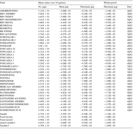
Table 8
GAPS: basic statistics (z=1,c=1%)
Fund Mean values over 16 quarters Whole period
No. gaps Mean gap Maximum gap Maximum gap Date
104 J.M. Chamorro,J.M-. P´erez de Villarreal / Insurance: Mathematics and Economics 27 (2000) 83–104
We have computed the value of the replicating portfolio at the end of each day over the 16 investment periods for each fund in the sample (c=1%). We thus know how many times during each period its value falls below the initial wealth, the size of each gap and hence the maximum of all of them.
Table 8 shows the results for each fund, by segments, and at a global level. The left part gives the average values when we consider the 16 quarterly periods individually. There seems to be a great similarity among types of funds concerning the occurrence of gaps: as an average, about half the days during the quarter the hedging portfolio does not fulfill its target; the average shortfall amounts to 4.55 per thousand, and as one would expect, it is slightly higher for equity funds than for bond funds. The differences among types widen when we come to the average maximum gap, ranging from 8.10‰for MFIFs to 9.01‰for VIFs.
The right part of the table takes all the periods at once so it deals with global maxima; it also shows the quarter when they occurred. Over the 4 years, the greatest failure in the hedging strategy goes from 2% of the initial wealth for some equity or variable income funds to approximately 1% for some FIFs; it generally happened during the second half of the year 1992.
Readers should judge for themselves whether these figures are daunting. The only thing we want to stress here is that the shortfalls do not seem to disturb the main purpose of the paper, namely, to rank funds.
References
Basak, S., 1995. A general equilibrium model of portfolio insurance. The Review of Financial Studies 4 8, 1059–1090. Benninga, S., Blume, M., 1985. On the optimality of portfolio insurance. Journal of Finance 40 (5).
Benninga, S., 1989. Numerical Techniques in Finance. MIT Press, Cambridge, MA.
Bird, R., Cunningham, R., Dennis, D., Tippet, M., 1990. Portfolio insurance: a simulation under different market conditions. Insurance: Mathematics and Economics 9, 1–19.
Bookstaber, R., Clarke, R., 1984. Option portfolio strategies: measurement and evaluation. Journal of Business 57 (4). Cox, J., Rubinstein, M., 1985. Options Markets. Prentice-Hall, Englewood Cliffs, NJ.
Gatto, M.A., Geske, R., Litzenberger, R., Sosin, H., 1980. Mutual fund insurance. Journal of Financial Economics 8, 283–317. Kahneman, D., Tversky, A., 1979. Prospective theory: an analysis of decision under risk. Econometrica 47, 263–291. Kendall, M.G., 1963. Rank Correlation Methods. Griffin, London.
Leland, H., 1980. Who should buy portfolio insurance? Journal of Finance 35 (2).
Leland, H., 1985. Option pricing and replication with transactions costs. Journal of Finance 40 (5). Rubinstein, M., 1984. Alternative paths to portfolio insurance. Financial Analysts Journal.
Sharpe, W., Alexander, G., Bailey, J., 1995. Investments, 5th Edition. Prentice-Hall, Englewood Cliffs, NJ. Siegel, S., 1956. Non-Parametric Statistics for the Behavioral Sciences. McGraw-Hill, New York.