Sharif University of Technology
Scientia IranicaTransactions E: Industrial Engineering www.scientiairanica.com
100% screening economic order quantity model under
shortage and delay in payment
B. Maleki Vishkaei
a, S.H.R. Pasandideh
b;and M. Farhangi
a a. Young Researchers and Elite Club, Qazvin Branch, Islamic Azad University, Qazvin, Iran. b. Department of Industrial Engineering, Faculty of Engineering, Kharazmi University, Tehran, Iran. Received 13 July 2013; received in revised form 1 November 2013; accepted 25 January 2014KEYWORDS Multiproduct; Economic order quantity; Screening;
Permissible delay in payment;
Discount; Shortage.
Abstract. For many years, the Economic Order Quantity (EOQ) model has been successfully applied to inventory management. This paper studies a multiproduct EOQ problem in which the defective items will be screened out by 100% screening process, and will be sold after the screening period. Delay in payment is permissible, though payment should be made during the grace period, and the warehouse capacity is limited. If not, there will be an additional penalty cost for late payment and the retailer will not be able to buy products at discount prices. All-units and incremental discounts are considered for the products which depend on order quantity, just like the permissible delay in payment. The Genetic Algorithm (GA) and the Particle Swarm Optimization (PSO) algorithm are used to solve the proposed model, and numerical examples are provided for better illustration. © 2014 Sharif University of Technology. All rights reserved.
1. Introduction
The basic economic order quantity model is expanded by researchers using dierent assumptions. Some of these assumptions seem to be more realistic and can be observed in real market environments. Retailers do not usually receive perfect goods and, conceivably, some defective items are found in their orders. The defect may be caused during the delivery process or by bad production. Porteus [1] studied the eect of defective items on an EOQ model in which the production process goes out of control considering a hypothesized probability. Wu and Ouyang [2] assumed the number of defective items as a random variable in a (Q,r,L) inventory model. They developed an algorithm procedure to obtain the optimal order quantity, the
or-*. Corresponding author. Tel.: +98 21 88830891; Fax: +98 21 88329213
E-mail addresses: [email protected] (B. Maleki Vishkaei); shr [email protected] (S.H.R. Pasandideh); [email protected] (M. Farhangi)
der point and the lead time. Shortages and permissible delays in payment are practical assumptions that help reach a tangible model. Economic order quantity under permissible delays in payment was studied by Goyal [3] for the rst time. Huang [4] studied a partial delay in payment, wherein the retailer pays the purchase cost at the end of the grace period in cases where the order quantity is more than the minimum amount of quantity, which leads to complete delay in payment. Otherwise, a part of the payment must be made as the order is lled. All-units discount and incremental discount are the policies that suppliers use to encourage retailers to increase their order size. Benton and Park [5] overviewed dierent purchase discounts and Weng [6] studied the all-units discount and incremental discount in inventory models, which were subsequently mentioned by many researchers.
of Salameh and Jaber [7] and gained optimal order and backorder quantities when shortage is permissible and completely backordered. Eroglu and Ozdemir [10] developed an EOQ model with shortages and defec-tive items that are categorized as imperfect quality and scrap items. Chang and Ho [11] revisited the model by Wee et al. [9] and used a renewal-reward theorem to obtain the expected prot per unit time. Kevin Hsu and Yu [12] considered a one-time only discount for Salameh and Jaber [7] model. They obtained the optimal order size, which is placed at a time when a price decrease is eective for three possible situations. Khan and Mehmood [13] studied an EOQ model considering errors in inspections and sales returns. In their model, the amount of returns was added to actual demands and was equal to perfect screened out items at a maximum to avoid shortage during the sales period. Hsu and Hsu [14] showed that there is an error in the model of Wee et al. [9], wherein the units that were backordered were shipped to customers before the screening process. They corrected the model and obtained the optimal order and backorder quantities using a renewal-reward theo-rem. This model was extended by Tai [15] considering two warehouses and using a multi screening process. Moreover, Hsu and Hsu [16] developed the model of Khan et al. [13], where the shortage is allowed and backordered. This paper further developed the model of Hsu and Hsu [14] by adding some new assumptions and considerations. As a result, it changed to a multi-product model. The mathematical model is later described in Sections 2 and 3. The genetic algorithm and the particle swarm optimization algorithm are used to solve the proposed model in Section 4, and these algorithms are then compared in the dierent examples in Section 5.
2. Notations and assumptions
The following notations and assumptions are used throughout this paper.
2.1. Notation
Qi: Order size of product i;
Di: Demand rate of product i;
xi: Screening rate for product i;
Ai: Ordering cost for product i;
pi: Average fraction of an order quantity
for product i, that is defective in Qi;
#i: Selling price per unit for product i;
Vi: Salvage value per defective item for
product i, Vi< ci;
di: Screening cost per unit for product i;
Bi: Maximum backordering quantity in
units for product i;
bi: Backordering cost per each unit of
product per unit of time for product i; i: Backordering cost per unit for product
i;
hi : Holding cost per each unit of product
per unit of time for product i; H : Length of planning horizon (in this
paper it is considered as one year), H = 1;
n : Number of products;
fi: Capacity of product i;
F : Total warehouse available space; i: Delay cost per unit of time for product
i;
Ti: Cycle time for product i;
Ni: Number of cycle times for product i,
Ni= H=Ti;
t1i: Length of cycle time for product i, in
which there is an inventory;
t2i: Length of cycle time for product i in
which there is no inventory; t3i: Time taken to ll Bi for product i;
ti: Length of cycle time for screening
product i;
k : Number of products that benet
all-units discount;
Mi: Permissible delay period for paying the
purchasing cost of product i to the supplier;
Ci: Unit purchasing cost without discount
of product i;
Ci;j: Purchasing cost per unit of product
i at the jth discount point; j = 1; 2; :::; m + 1;
Mi;j : Permissible delay time for product i at
the jth discount point;
u : An innite number;
T Si: Ordering cost per cycle for product i;
T Bi: Shortage cost per cycle for product i;
T Hi: Holding cost per cycle for product i;
T Mi: Delay cost of product i;
T P0
i : Purchasing cost per cycle for product i
considering discount; T P00
i : Purchasing cost per cycle for product i
T Pi : Purchasing cost per cycle for product i;
T Ri: Revenue per cycle for product i;
T P V : TotalNetProt value per cycle.
si=
8 < :
1; If product i receives discount (T Mi= 0)
0; Otherwise (T Mi > 0)
Decision variables:
Qi: Order quantity of product i;
Bi: Maximum shortage (backorder) level
of product i. 2.2. Assumptions
1. Replenishment is instantaneous.
2. Shortage is allowed and will be backordered in the next period.
3. 100% screening process is used and screening rate is greater than demand rate (xi> Di).
4. Defective items are sold at price Vi, subsequently,
the screening process is nished.
5. The supplier demands the cost of each product batch in just one payment, and, since the retailer pays for his current costs, like holding costs, during the cycle time, the purchasing cost occurs at the end of the selling period when all the goods are sold (when the inventory level reaches zero). Therefore, the payment may occur during or after the grace period and hinges on the cycle time.
6. There are all-units discount and incremental dis-count policies for the products.
7. Permissible delay in payment hinges on order quan-tity. If the payment occurs in the permissible time, the retailer benets from discount prices. Other-wise, not only are discount prices not considered for him, he will be charged a fee for lateness, as a delay cost.
3. Mathematical model
Figure 1 depicts the inventory model in which the shortage is satised in each cycle at a rate of xi(1
pi) Di, after that the time period t3i, the shortage
is completely backordered. According to Hsu and Hsu [13], Bi+ t3iDi = xi(1 pi)t3i =xBi(1 pixi(1 pi) Di)i and
t1i; t2i; t3i are parts of the cycle with no shortage, the
part of the cycle with shortage, and the time taken to ll Bi instantaneously, which can be shown as:
t1i= Qi(1 pDi) Bi
i ; (1)
t2i= BDi
i; (2)
Figure 1. Behavior of the proposed inventory model. Table 1. The amounts of Mi and Ci depend on the order
quantity.
Qi Mi Ci
qi;0< Qi qi;1 Mi;1 Ci;1
qi;1< Qi qi;2 Mi;2 Ci;2
... ... ...
qi;m 1< Qi qi;m Mi;m Ci;m
qi;m< Qi Mi;m+1 Ci;m+1
t3i= x Bi
i(1 pi) Di: (3)
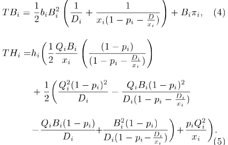
Eqs. (4) and (5) calculate shortage cost and the holding cost per cycle:
T Bi= 12biBi2 D1 i +
1 xi(1 pi xDi)
!
+ Bii; (4)
T Hi=hi
1 2
QiBi
xi
(1 pi)
(1 pi Dxii)
!
+12
Q2
i(1 pi)2
Di
QiBi(1 pi)2
Di(1 pi Dxii)
QiBi(1 pi)
Di +
B2
i(1 pi)
Di(1 pi Dxii)
+piQ2i
xi
: (5)
Ordering cost per cycle is Ai and the price discount
and permissible delay in payment depend on the order quantity. Table 1 shows the relationship between them. In this table:
qi0= 0; 0 < Mi;1< Mi;2< ::: < Mi;m+1;
and:
Ci;1> Ci;2> ::: > Ci;m+1:
between TV set models and only depends on the price of the merchandise.
The retailer is not able to pay the supplier before selling all units in each period, and the payment may occur during or after the grace period. Therefore, there will be a delay cost if the inventory level reaches zero after the grace period, due to non-payment within the dened period and delay in payment. In this case, the retailer is not allowed to benet from discount prices, and delay cost equals Eq. (6). When the inventory level reaches zero before nishing the grace period (all the products of type i are sold and the retailer can pay the purchasing cost before the grace period is nished), T Mi= 0 and the retailer can benet from the discount
price. Moreover, Miand Cican be gained from Table 1.
They can be replaced byPm+1j=1 yi;jMi;j,Pm+1j=1 yi;jCi;j
in which yi;j is a binary variable and Pm+1j=1 yi;j = 1.
Therefore, T Mi can be summarized to Eq. (7).
T Mi=
The rst k products receive an all-units discount and the incremental discount is considered for the others. As mentioned before, the retailer can benet from the discount only when the payment occurs within the grace period. Unit price can be obtained from Table 1. When Mi< t1i, the retailer has to pay the purchasing
cost with no discount:
T P00
i = QiCi;1; i = 1; 2; :::; n: (8)
When Mi t1i, the retailer can use discount prices
and the purchasing cost can be formulated as:
T p0
Therefore, the purchasing cost per cycle can be ob-tained as:
T Pi= T Pi0si+ T Pi00(1 si); i = 1; 2; :::; n:
The revenue per cycle is:
T Ri= (1 pi)Qi#i+ piQiVi; i = 1; 2; :::; n:
The net prot value that the retailer earns per cycle is:
T P V =Xn
i=1
[T Ri (T Si+T Pi+T Mi+T Hi+T Bi)] ;
i = 1; 2; :::; n:
The objective is to maximize the net prot value per cycle, and the mathematical model becomes:
T Mi
Eqs. (11), (12) and (13): Calculation of the purchasing cost for an all-unit discount, an incremental discount and purchasing cost when Mi t1i:
Eq. (14): Calculation the revenue per cycle; Eq. (15): Calculation the holding cost per cycle; Eq. (16) and (17): Find the amounts of binary variable for dening Mi and Ci.
Eqs. (19) and (20): These two constraints together dene:
Eq. (21): The warehouse capacity is limited.
4. Solving algorithms
The mathematical model mentioned is a constrained nonlinear-programming model, and the number of constraints depends on the number of products. The greater the number of products, the more constraints are faced, which makes the problem more complicated, and more time is needed for solution. In this paper, the genetic algorithm and the Particle Swarm Optimization (PSO) algorithm are used to solve the proposed model and numerical examples are given to clarify their workability.
4.1. Genetic algorithm
The genetic algorithm was proposed by J. Holland [17]. This algorithm starts with a random population in which infeasible chromosomes are vanished and re-produced. Each chromosome has two rows; the rst indicating order quantities and the second indicating shortages. Eq. (22) shows the proposed chromosome:
Chromosome =
Other populations are created via elitism, crossover and mutation. A specic number of generations are considered as the algorithm stopping criteria. To avoid producing infeasible siblings which contain columns in which the amount of shortage is greater than the order quantity, the crossover and mutation operations are performed on the columns of the chromosomes. Eqs. (23) to (28) show how these operations work. In Eqs. (23)-(25), the random-crossover-mask denes how to select columns from the parents. For example, if the second number is 0, then the son chromosome's second column is equal to the father chromosome's second column. In Eqs. (26)-(28), the mutation percentage is considered 0.1 and the columns, whose corresponding elements in the random matrix are less than 0.1, will be regenerated according to Bi< Qi.
Eqs. (23)-(25) show the performance of the crossover operation:
Eqs. (26)-(28) show the performance of the mutation operation:
4.2. Particle swarm optimization
solution so far reached by the particle (personal best) and the best current solution obtained so far by any particle (global best). A specic number of iterations are considered for the stopping criteria and the last global best will be the nal solution of the algorithm.
5. Numerical examples
After tuning the two proposed algorithm's parameters, a small size example is solved by Lingo and the result is compared to GA and PSO algorithms. The proposed example parameters are shown in Tables 2 and 3. In this example, the maximum capacity is considered to be 1000; the rst product benets the all-units discount and other products benet from incremental discounts. As shown in Table 4, GA and PSO do not reach the optimal solution, but GA's answer was closer to Lingo's answer and the running time of GA was less
Table 2. Small example purchasing costs and permissible delay times.
Qi C1 C2 C3 Mi
0 < Qi 200 99 96 80 0.1
200 < Qi 400 91 89 72 0.2
400 < Qi 73 52 55 0.4
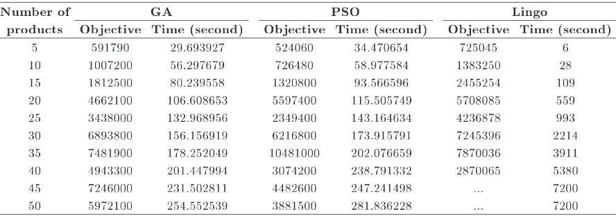
than the running time of PSO. On the other hand, the single optimal solution can be obtained by Lingo when the problem is small. The scale of the model mainly depends on the number of constraints, which increases with the number of products. Therefore, to solve large problems, GA and PSO algorithms are used. As shown in Table 5, Lingo had a longer running time than the heuristic algorithms when the number of the products became more than 10 (500 iterations are considered the stopping criteria for heuristic algorithms). Moreover, Lingo obtained a local optimum for examples with 35 and 40 products, and it could not gain an answer for examples with 45 and 50 products after 7200 seconds. Comparing heuristic algorithms, the computational time of GA is better than PSO in all examples. Moreover, GA gained a better objective for most of the examples and PSO worked better in examples with 20 and 35 products.
6. Conclusions
In this paper, an inventory model was studied con-sidering defective items and their shortages, which are backordered. Screening rate is always greater than demand rate and all products are sold only after a screening process. There is a delay in payment,
Table 3. Small example parameters.
Product Di pi hi Ai bi i i fi xi #i Vi di
1 1000 0.2 0.4 194 18 20 24 5 8200 222 112 10
2 2200 0.3 0.6 165 16 11 37 6 9400 235 122 6
3 1800 0.15 0.3 125 13 11 22 4 9000 242 130 8 Table 4. Results of small example.
Solving method Q1 Q2 Q3 B1 B2 B3 Objective Time (second)
Lingo 1.25 1.429 246.29 1 1 1 35878.93 1
GA 41.49 6.63 187.39 5.36 3.37 33.38 31082 27.961231
PSO 67.8342 19.6408 135.57 3.701 7.94 18.20 27740 32.798773 Table 5. Comparison of GA and PSO solutions.
Number of GA PSO Lingo
products Objective Time (second) Objective Time (second) Objective Time (second)
5 591790 29.693927 524060 34.470654 725045 6
10 1007200 56.297679 726480 58.977584 1383250 28
15 1812500 80.239558 1320800 93.566596 2455254 109
20 4662100 106.608653 5597400 115.505749 5708085 559
25 3438000 132.968956 2349400 143.164634 4236878 993
30 6893800 156.156919 6216800 173.915791 7245396 2214
35 7481900 178.252049 10481000 202.076659 7870036 3911
40 4943300 201.447994 3074200 238.791332 2870065 5380
45 7246000 231.502811 4482600 247.241498 ... 7200
which depends on the order quantity, and the retailer is able to benet from discount prices only in cases where payment occurs during the grace period. After describing the mathematical model, a small example is solved by Lingo and the optimal solution is gained. As the number of products increases, the number of con-straints and the scale of the problem will change. Lingo can only gain local optimum solutions after a longer running time. Therefore, for large scale problems, GA and PSO algorithms are used and compared to each other, considering 10 dierent problems. Numerical examples indicated that GA has a better performance for the proposed model. GA solved the examples in less time and achieved better solutions for most of them.
References
1. Porteus, E.L. \Optimal lot sizing, process quality improvement and setup cost reduction", Oper. Res., 34(1), pp. 137-144 (1986).
2. Wu, K.S. and Ouyang, L.Y. \(Q,r,L) inventory model with defective items", Comput. and Ind. Eng., 39(1), pp. 173-185 (2001).
3. Goyal, S. \Economic order quantity under conditions permissible delay in payments", J. of the Oper. Res. Soc., 36, pp. 335-338 (1985).
4. Huang, Y.F. \Economic order quantity under condi-tionally permissible delay in payments", Eur. J. of Oper. Res., 176(2), pp. 911-924 (2007).
5. Benton, W. and Park, S. \A classication of literature on determining the lot size under quantity discounts", Eur. J. of Oper. Res., 92(2), pp. 219-238 (1996). 6. Weng, Z.K. \Modeling quantity discounts under
gen-eral price-sensitive demand functions: Optimal policies and relationships", Eur. J. of Oper. Res., 86(2), pp. 300-314 (1995).
7. Salameh, M.K. and Jaber, M.Y. \Economic order quantity model for item with imperfect quality", Int. J. of Prod. Econ., 64(1), pp. 59-64 (2000).
8. Cardenas-Barron, L.E. \Observation on economic pro-duction quantity model for items with imperfect qual-ity", Int J. of Prod. Econ., 67(2), pp. 201-201 (2000). 9. Wee, H.M., Yu, J. and Chen, M.C. \Optimal inventory model for items with imperfect quality and shortage backordering", Omega, 35(1), pp. 7-11 (2007). 10. Eroglu, A. and Ozdemir, G. \An economic order
quantity model with defective items and shortages", Int. J. of Prod. Econ., 106(2), pp. 544-549 (2007). 11. Chang, H.C. and Ho, C.H. \Exact closed-form
so-lutions for optimal inventory model for items with
imperfect quality and shortage backordering", Omega, 38(3), pp. 233-237 (2010).
12. Kevin Hsu, W.K. and Yu, H.F. \EOQ model for imperfective items under a one-time-only discount", Omega, 37(5), pp. 1018-1026 (2009).
13. Khan, M., Jaber, M. Y. and Bonney, M \An economic order quantity (EOQ) for items with imperfect quality and inspection errors", Int. J. of Prod. Econ., 133(1), pp. 113-118 (2011).
14. Hsu, J.T. and Hsu, L.F. \A note on, optimal inventory model for items with imperfect quality and shortage backordering", Int. J. of Ind. Eng. Comput., 3(5), pp. 939-948 (2012).
15. Tai, A.H. \An EOQ model for imperfect quality items with multiple screening and shortage backordering", arXiv Preprint arXiv, pp. 1302-1323 (2013).
16. Hsu, J.T. and Hsu, L.F. \An EOQ model with imper-fect quality items, inspection errors, shortage backo-rdering, and sales returns", International Journal of Production Economics (2013).
17. Holland, J., Adaptation in Natural and Articial Sys-tems, The University of Michigan Press (1997). 18. Kennedy, J. and Eberhard, R.C. \Particle swarm
optimization", In Proc. IEEE Int. Conf. on Neu-ral Networks, Piscataway, NJ, USA., pp. 1942-1948 (1995).
Biographies
Behzad Maleki Vishgahi received his BS and MS degrees in Industrial Engineering from the Islamic Azad University, Qazvin, Iran. His research interests include areas of inventory control and supply chain management.
Seyed Hamid Reza Pasandideh received his BS, MS and PhD degrees, all in Industrial Engineering, from Sharif University of Technology, Tehran, Iran, in 1994, 1998 and 2005, respectively. He is currently Assistant Professor in the Industrial Engineering De-partment at Kharazmi University, in Iran. His research interests include applications of operations research in production planning and inventory control. More specically, he is studying mathematical modeling and solution methods, including exact procedures.