Neurális hálózatok alkalmazása az ökológiai adatok értékelésében

Egyetemi doktori (PhD) értekezés NEURAL NETWORKS IN ECOLOGICAL DATA ANALYSIS NEURÁLIS HÁLÓZATOK ALKALMAZÁSA AZ ÖKOLÓGIAI ADATOK ÉRTÉKELÉSÉBEN Várbíró Gábor Témavezetők: Dr. Tóthmérész Béla Dr. Borics Gábor. DEBRECENI EGYETEM Juhász-Nagy Pál Doktori Iskola Debrecen, 2009.

A doktori értekezés betétlapja Ezen értekezést a Debreceni Egyetem TTK ................Doktori Iskola … Kvantitatív és Terresztris Ökológia …programja keretében készítettem a Debreceni Egyetem TTK doktori (PhD) fokozatának elnyerése céljából.. Debrecen, 2009. június. 25. ………………………… a jelölt aláírása. Tanúsítom, hogy ....Várbíró Gábor.......................... doktorjelölt 2000- 2009. között, a fent megnevezett Doktori Iskola Kvantitatív és Terresztris Ökológia programjának keretében irányításommal végezte munkáját. Az értekezésben foglalt eredményekhez a jelölt önálló alkotó tevékenységével meghatározóan hozzájárult. Az értekezés elfogadását javasolom. Debrecen, 2009. június 25. .………………………..… a témavezető aláírása. Tanúsítom, hogy ....Várbíró Gábor.......................... doktorjelölt 2000- 2009. között, a fent megnevezett Doktori Iskola Kvantitatív és Terresztris Ökológia programjának keretében irányításommal végezte munkáját. Az értekezésben foglalt eredményekhez a jelölt önálló alkotó tevékenységével meghatározóan hozzájárult. Az értekezés elfogadását javasolom. Debrecen, 2009 június 25. ……………………….…… a témavezető aláírása.

NEURAL NETWORKS IN ECOLOGICAL DATA ANALYSIS NEURÁLIS HÁLÓZATOK ALKALMAZÁSA AZ ÖKOLÓGIAI ADATOK ÉRTÉKELÉSÉBEN Értekezés a doktori (Ph.D.) fokozat megszerzése érdekében készült, a Természettudományi tudományágban. Írta: …Várbíró Gábor... okleveles Biológus-ökológus Készült a Debreceni Egyetem … Juhász-Nagy Pál Doktori Iskola Kvantitatív és Terresztris Ökológia programja keretében Témavezetők: Dr. Tóthmérész Béla Dr. Borics Gábor A doktori szigorlati bizottság: elnök: Dr. Nagy Sándor Alex tagok: Dr. Magura Tibor Dr. Nagy Miklós A doktori szigorlat időpontja: 2007. június 14.. ………………………… ………………………… ………………………… ………………………… …………………………. Az értekezés bírálói: ………………………… …………………………. ………………………… …………………………. A bírálóbizottság: elnök: ………………………… tagok: ………………………… ………………………… ………………………… …………………………. ………………………… ………………………… ………………………… ………………………… …………………………. Az értekezés védésének időpontja: 2009… . ……………… … ..

Neural networks in ecology. 1. CONTENTS Papers included........................................................................................................ 2 Introduction and Objectives................................................................................... 3 Material and methods ............................................................................................. 9 1.1 Statistical methods .......................................................................................... 9 SOM algorithm ................................................................................................. 9 Structuring index (SI) ..................................................................................... 12 Clustering of the SOM .................................................................................... 14 1.2 Ecological Databases .................................................................................... 16 Results..................................................................................................................... 19 Summary ................................................................................................................ 30 Összefoglalás .......................................................................................................... 31 Acknowledgements ................................................................................................ 41 Köszönetnyílvánítás............................................................................................... 42 References .............................................................................................................. 43 Publications of Gábor Várbíró............................................................................. 48 1.1 Publications connected to the theses ............................................................. 48 1.2 Other publications ......................................................................................... 48 1.3 Oral presentations and posters ...................................................................... 49 Paper 1.......................................................................................................................I Paper 2..................................................................................................................... II Paper 3....................................................................................................................III Paper 4.................................................................................................................... IV Paper 5......................................................................................................................V.

Neural networks in ecology. 2. Papers included 1. Várbíró, G., Ács, É., Borics, G., Érces, K., Fehér, G., Grigorszky, I., Japport, T., Kocsis, G., Krasznai, E., Nagy, K., Nagy-László, Zs., Pilinszky, Zs., Kiss, K.T. (2007): Use of Self-Organizing Maps (SOM) for characterisation of riverine phytoplankton associations in Hungary. - Arch. Hydrobiol. Suppl. Large Rivers 17: 383-394. (Printed with kind permission from the Journal of Arch. Hydrobiol) 2. Várbíró, G., Borics, G., Kiss, K.T., Szabó, K. É., Ács, É. (2007): Use of Kohonen Self Organizing Maps (SOM) for the characterisation of benthic diatom associations of the River Danube and its tributaries. – Arch. Hydrobiol. Suppl. Large Rivers 17: 395-403. (Printed with kind permission from the Journal of Arch. Hydrobiol) 3. Ács, É., Borsodi, A.K., Kiss, É., Kiss, K.T., Szabó, K.É., Vladár, P., Várbíró, G., Záray, Gy. (2008): Comparative algological and bacteriological examinations on biofilms developed on different substrata in a shallow soda lake – Aquat Ecol (2008) 42:521–531. (Printed with kind permission from the Journal of Aquatic Ecology) 4. Borics, G., Várbiró, G., Grigorszky, I., Krasznai, E., Szabó, S., Kiss, K. T. (2007): A new evaluation technique of potamoplankton for the assessment of the ecological status of rivers. Arch. Hydrobiol. Suppl. Large Rivers 17: (3-4) 465-486. (Printed with kind permission from the Journal of Arch. Hydrobiol) 5. Van Dam, H., Stenger-Kovács, Cs., Ács, É., Borics, G., Buczkó, K., Hajnal, É., Soróczki-Pintér, É., Várbíró, G., Tóthmérész, B., Padisák, J. (2007): Implementation of the European Water Framework Directive: Development of a system for water quality assessment of Hungarian running waters with diatoms. - Arch. Hydrobiol. Suppl. Large Rivers 17: 339-364. (Printed with kind permission from the Journal of Arch. Hydrobiol).

Neural networks in ecology. 3. Introduction and Objectives “in the 19 century the data speak for itself, at present its completely different …”. The need for better techniques, tools and practices to analyse ecological and economic systems within an integrated framework at wider scales has never been so great. Currently, individuals of different professions consider scientific predictions that are based on highly complicated principles and hypotheses as beyond their comprehension and often ignore them (Clark et al., 2001). Scientists are becoming more focused on science and research of course than improving their communication with the general public (Buckeridge, 2001). The transformation of large quantities of disparate data into simple, useable information is seen as a major challenge in many current environmental monitoring programmes. Vant (1999) identified two key aspects of this, namely, the identification of robust methods to summarise large volumes of data without losing the useful information in it, and presenting this information to a largely non-technical audience in an understandable and compelling manner. The task of transforming data into useful information is a major challenge to environmental scientists, who were probably attracted to the study of ecosystems because of the complexity involved, and now increasingly find themselves having to move beyond the security of complicate conceptual models and the jargon of the highly technical journals, to communicate with a wider community. Over the last few years, the use of Artificial Neural Network (ANN) techniques has provided ecologists with a powerful method for modelling large volumes of ecological data (Paisley et al., 2003).Neural networks are powerful computational tools that can be used for classification, pattern recognition, empirical modelling and for many other tasks. Neural networks can be "trained" to provide the right.

Neural networks in ecology. 4. output (binary, fuzzy, quantitative) if enough input-output patterns are available and if these patterns effectively describe the system that is to be modelled. The earliest work in neural computing goes back to the 1940's when McCulloch and Pitts (McCulloch and Pitts, 1943) introduced the first neural network computing model. Reinforcing this concept of neurons and how they work was a book written by Donald Hebb. The Organization of Behavior was written in 1949 (Hebb, 1949). It pointed out that neural pathways are strengthened each time that they are used. In the 1950's, Rosenblatt's (Rosenblatt, 1956, 1957) work resulted in a two-layer network, the perceptron, which was capable of learning certain classifications by adjusting connection weights. The architecture inspired by the human brain which contains neuron connected to each other by synapses. The artificial analogue of the neuron is the perceptron. (Fig. 1.). Fig. 1. The structure of the natural neuron and the artificial perceptron Although the perceptron was successful in classifying certain patterns, it had a number of limitations, which the decline of the field of neural networks. However, the perceptron had laid foundations for later work in neural computing. In the early 1980's, researchers showed renewed interest in neural networks. These studies show promising results in modelling complex relationships between biological and environmental variables of natural habitats to support sustainable environment development (Shanmuganathan, 2005). Bayesian belief networks and ANN techniques, namely back propagation and self organizing maps (SOM), were found to be successful in calculating a set of biotic indices for.

Neural networks in ecology. 5. monitoring of river quality based on the distribution and abundance of macroinvertebrate taxa and environmental parameters of 1995 national survey data (Walley et al., 1998). The study concluded that the methods tested to have shown considerable potential for use in river quality classification and river management. Modelling Patterns in Environmental Data (MOPED) uses SOM techniques for modelling patterns within fish species distribution and elevation of sampled freshwater systems in a region (Jowett, 2001). MOPED also was found to be capable of predicting the biological assemblages that should be present in certain streams. Onkal-Engin et al. (2005) successfully applied a back-propagation ANN algorithm to develop an electronic nose for the purpose of controlling sewage odours in wastewater treatment plants. Ecosystem analysis and prediction with empirical statistical and analytical methods are often limited by the spatial complexity and temporal dynamic character of ecological processes. This is one reason for the typically non-linear interrelations of variables and species with data being not normally distributed. Artificial neural networks provide an attractive alternative tool for analysing ecological data and for modelling due to their specific features such as non-linearity, adaptivity, generalisation and model independence (no a-priori model needed). ANNs have been applied to various fields of aquatic sciences and engineering, such as modelling water quality (e.g. Daniell and Wundke, 1993; Maier and Dandy, 1996a,b; 1997; Lachtermacher and Fuller, 1994; Schizas et al., 1994; Maier, 1995; Winkler and Voigtlander, 1995; Kaluli et al., 1998; Wen and Lee, 1998) and relating community characteristics with environmental variables (e.g. Chon et al., 1996; Lek et al., 1996; Recknagel, 1997; Recknagel et al., 1997, 1998; Guegan et al., 1998; Lee et al., 1998; Maier et al., 1998). An important aspect of an ANN model is whether it needs guidance in learning or not. Based on the way they learn, all artificial neural networks can be divided into two learning categories - supervised and unsupervised. In supervised learning, a desired output result for each input vector is required when the network is trained..

Neural networks in ecology. 6. An ANN of the supervised learning type, such as the multi-layer perceptron, uses the target result to guide the formation of the neural parameters. It is thus possible to make the neural network learn the behaviour of the ecological system. In unsupervised learning, the training of the network is entirely data-driven and no target results for the input data vectors are provided. An ANN of the unsupervised learning type, such as the self-organizing map, can be used for clustering the input data and find features inherent to the problem. (Burke, and Ignizio, 1992) The biological monitoring of the water currents in several countries provided large volume datasets during the last decades. In case of large volume of data, the traditional multivariate statistical methods like cluster analysis and ordination is difficult to interpret and present the information. Self Organizing Map is a novel approach for the visualization of high-dimensional data. Self-organizing Map is a data visualization technique invented by Professor Teuvo Kohonen which reduces the dimensions of data through the use of self-organizing neural networks. SOM converts complex statistical relationships between high-dimensional data items into simple geometric relationships on a low-dimensional display. Thus, it compresses information while preserving the most important topological and metric relationships of the primary data items (Kohonen 2001). The main advantages of the SOM are the better data visualisation and noise reduction (Vesanto and Alhoniemi 2000). Mangiameli et al. (1996) compared SOM and several hierarchical clustering methods, and found SOM superior to hierarchical clustering in both robustness and accuracy. In addition, the two-level clustering approach (SOM neural network followed by K-means clustering) was developed and successfully applied to cluster data (Vesanto and Alhoniemi 2000; Beccali et al. 2004). SOMs are increasingly popular tools in ecology, and have been used to describe bentic algal assemblages in France and Luxembourg (Gosselain et al. 2005, Rimet et al. 2005a, 2005b). The self-organizing map (SOM) is an efficient tool for mining nonlinear data and has been extensively used for patterning community data since 1990s (e.g., Chon et al., 1996, Giraudel et al., 2000, Kwak et al., 2000; Levine et.

Neural networks in ecology. 7. al., 1996; Park et al., 2003, 2005). Chon et al. (1996) classified benthic macroinvertebrate communities in polluted streams with the SOM and elucidated community patterning according to anthropogenic disturbances and locality of the sample sites. Chon et al. (2002) further implemented the SOM to a large-scale data collected in different river systems in the Korean Peninsula for 16 years. The largescale data were accordingly arranged to reveal the impact of environmental disturbances. In this study, we further elaborated to show the trained SOM as a means of providing a comprehensive view on ecological states of the communities and to use the SOM as a tool for assessing biological water quality. Further articles which summarise the application of the SOM in ecological application( Kaski et al., 1996, Kalteh et al.,2008, Ceregrino and Park, 2009) The Hungarian routine monitoring program for chemical parameters has been monitored in running and standing waters for more than 40 years already. Unfortunately in the early years the only two biological components which were stored in a database were the index value and the chlorophyll-a content of the given samples. In 2000 the author of the theses started to build a database for storing the taxa list in digital form. Since then the system became the part of the Hungarian monitoring program. In 2001 there has been an initial start in the qualitative monitoring of macroinvertebrates, as a first step towards implementation of the Water Framework Directive (European Union, 2000) requirements. In 2005 other biological elements of the WFD were involved in the national monitoring program such as phytobenton and macrophytes. At present all of these biological quality elements have a relevant database to store the taxalist and sampling event features. From the presented publications the author’s main interests and responsibilities, as well as the main goals of the PhD thesis were the followings: Characterize selected Hungarian running waters according to their characteristic phytoplankton assemblages with the help of SOM techniques (Paper 1).

Neural networks in ecology. 8. Construction of useable biological database for storing relevant ecological information on phytoplankton and phytobenton biological elements (Paper 4, 5) Characterize the upper Danube section based on their characteristic diatom communities by SOM methods (Paper 2) Describe the differences and similarities of the periphyton of Lake Velencei on different substrate using SOM statistics (Paper 3) ..

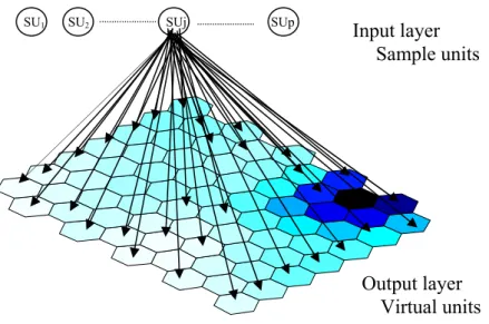
Neural networks in ecology. 9. Material and methods “Gagnants and Perdants”. 1.1 Statistical methods SOM algorithm For statistical analysis in Paper 1, 4 and 5 we used the SOM algorithm which can make a projection of the database into a two dimensional hexagonal map. Closely related communities were placed into neighbouring hexagons by their similarities, while samples with different communities were in distant hexagons. The SOM can display the groupings of samples and species together; therefore, each species can be evaluated by its importance (Kohonen, 2001). The SOM Toolbox (http://www.cis.hut.fi/projects/somtoolbox) was used to implement the SOM under a MATLAB™s environment. In this chapter I would describe the algorithm in details. We followed the abbreviations of the publication Giraduel (Giraduel and Lek , 2001). The SOM consists of two layers: input and output layers connected by connection intensities (weights).(Fig. 2.) SU1. SU2. SUj. SUp. Input layer Sample units. Output layer Virtual units Fig. 2. The structure of the SOM neural network Input layer gets information from data matrix, while output layer visualizes the computational results. When an input vector is sent through the network, each neuron of the network computes the distance between the weight vector and the input vector. The output layer consists of output neurons, which are usually.

Neural networks in ecology. 10. arranged into a two-dimensional grid for better visualization. The best arrangement for the output layer is a hexagonal lattice, as it does not favour horizontal and vertical directions as much as a rectangular array (Kohonen, 2001). The ecological data usually contains a matrix of sample units (SU) and species composition data as like in table 1.. Sample units. Table 1.An ecological data matrix, i species (sp1,…, spi) are observed in SUp sample units (SU1,…, SUp), Xip species weight (like abundance etc.). SU1 SU2. Sp1 X11 X12. Species / variables/ ------------------Spi ------------------Xi1 ------------------Xi2. SUp. X1p. -------------------. Xip. This is the input layer of the SOM. The goal of the SOM is to make the output layer consist of virtual units (VU) with the virtual species weight (prototype vector or codebook vector) as seen in table .2.. Virtual units. Table 2. .The SOM data matrix, i species (sp1,…, spi) are observed in VUp virtual units (VU1,…, VUp), Wip weight vector (species abundance etc). VU1 VU2. Sp1 W11 W12. Species / variables/ ------------------Spi ------------------Wi1 ------------------Wi2. VUp. W1p. -------------------. Wip. The algorithm of the SOM process can be described as: • Step 1: Epoch t=0, the virtual units VUp are initialized, weights drawn from the input dataset. • Step 2: A sample unit SUj is randomly chosen as an input unit. • Step 3: Using some metric, the distances between SU and each virtual unit are computed. • Step 4: The virtual unit VUc closest to the input SUj is chosen as the winning neuron. VUc is called the Best Matching Unit (BMU). • Step 5: The virtual units VUp are updated with the learning rule: • Step 6: Increase time t to t+1. If t<tmax then go to step 2 else stop the training..

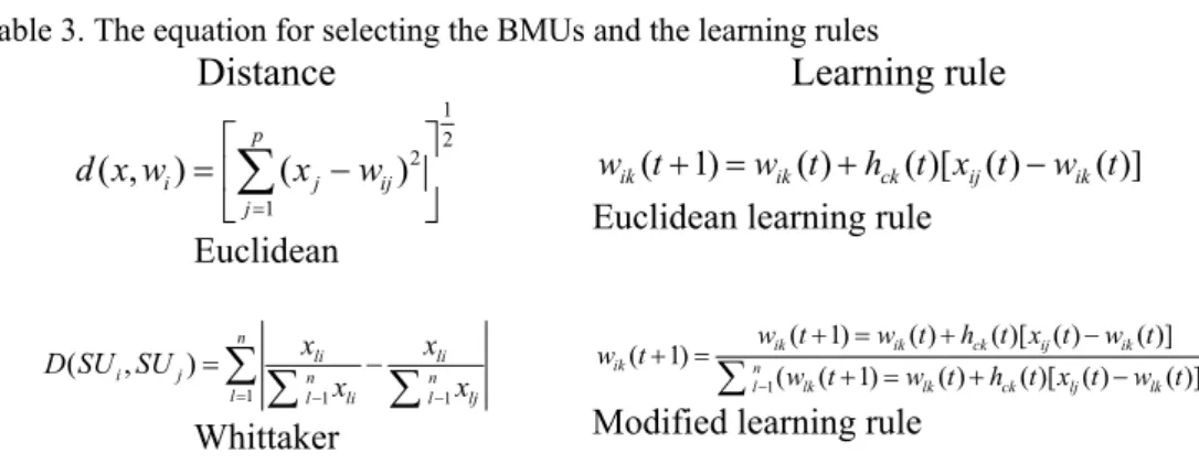
Neural networks in ecology. 11. In step 1, the user decide the size of the map, this is an important question because if the map is too big there would be empty cells in the final map, whereas if the size is too small there would be less distinct groups as expected. The optimal numbers of nodes according to Vesanto (Vesanto, 2000) can be calculated as:. Nn = 5 SU d Where Nn is the number of nodes in the final map and SUd is the number of sample units. There are two ways to initialize the weight vectors. The first is to give each weight vector a random value based on the SU, the second is to make a linear gradient from the weights. In step 3, the distance or the measure of dissimilarity between stations can be chosen. Usually the conventional Euclidean distance is widely usable but is not the only possibility. Some measurements that take into account the difficult problems of double zero or scale (e.g. binary data) can also be used. However, the use of the learning rule has to be made very prudently. If Euclidean distance is not used, the learning equation has to be adapted in order to be compatible with the chosen distance or the measure of dissimilarity (Kaski, 1997). For instance Giraudel and Lek (2001) used the Whittaker’s relative transformation for absolute distance (Whittaker, 1952), as suggested by Orlóci (1978) in this way the learning rule should also change as seen in table 3. Table 3. The equation for selecting the BMUs and the learning rules. Distance. Learning rule. ⎤ ⎡ p d ( x, wi ) = ⎢∑ ( x j − wij ) 2 ⎥ ⎦ ⎣ j =1 Euclidean n. D( SU i , SU j ) = ∑ l =1. ∑. xli n l −1 li. x. Whittaker. −. ∑. 1 2. wik (t + 1) = wik (t ) + hck (t )[ xij (t ) − wik (t )]. Euclidean learning rule. xli n l −1 lj. x. wik (t + 1) =. ∑. w (t + 1) = wik (t ) + hck (t )[ xij (t ) − wik (t )]. ik n l −1. ( wlk (t + 1) = wlk (t ) + hck (t )[ xlj (t ) − wlk (t )]). Modified learning rule. In step 5, in the Euclidean learning rule the function hck(t) is the neighbourhood function. During the learning process, the BMU defined in step 4 is not the only updated unit. In the grid, a neighbourhood is defined around the BMU and all units within this neighbourhood are also updated. Several choices can be made for the definition of the neighbourhood function (see Kohonen, 2001). The most often neighbourhood is the Gaussian function:.

Neural networks in ecology. 12. ⎛ rk − rc 2 ⎞ ⎟ hck (t ) = α (t ) ⋅ exp⎜ − ⎜ 2σ 2 (t ) ⎟ ⎝ ⎠ ||rk – rc || is the Euclidean distance on the map between the winning unit VUc and each virtual unit VUk. σ is a decreasing function of time, which defines the width of the part of the map, affected by the learning. α is the ‘learning-rate factor’, Both factors are decreasing functions of the time and converge towards 0. The learning is broken down into two parts: 1. the ordering phase: during this phase, the virtual stations are widely modified in a large neighbourhood of the BMU with large values of α and σ 2. the tuning phase: when this second phase takes place, only the virtual units adjacent of the Best Matching Unit are modified. This phase is much longer than the former one and σ is decreasing very slowly towards 0. It is recommended that the number of steps in the tuning phase has to be 500 times the number of units in the output layer. When the learning process is finished, a map with S hexagons is obtained and in each hexagon, there is a virtual station in which the weights/species composition has been computed. Then, this map can be visualised in different ways: • The sample units can be mapped. The BMU is computed for each sample unit and label the corresponding hexagon. • The species composition of each virtual unit can display the distribution of each weights/species. The SOM map of the variables called component planes • The two presentations can be mixed to display the sample units and the weights/species distribution on the same map.. Structuring index (SI) In order to characterise the VU groups we used the Structuring Index (SI) which was originally developed to define the species that show the strongest influence on the organization of the SOM map (Park et al., 2005). Tison et al. (2004, 2005) used the SI to evaluate relevant diatom species in the classification of diatom communities. The set of species showing high SI can be considered as the indicator species. Taxa showing strong gradient display have high SI values, whereas species showing weak gradient present low SI values. Thus, the higher the value of SI, the more relevant the variable is to the structure of the map. The index calculation based on the weight vectors of the SOM see Fig. 3..

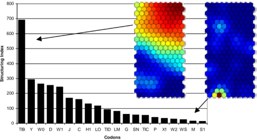
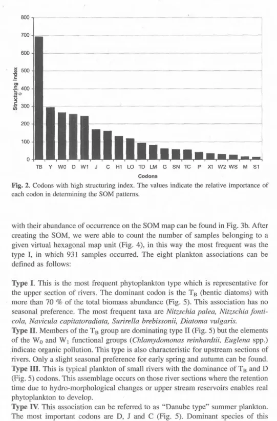
Neural networks in ecology. 13 S. j −1. SI i = ∑∑ j =1 k =1. Wij − Wik r j − rk. This equation calculates the SI value, where wij and wik are the connection weights of the ith species in the SOM units, ||rj−rk|| is the topological distance between units j and k , S is the total number of SOM output unit. Fig. 3. topological distance of the SOM output units used in the SI calculation Then based on the SI value of each variable it is possible to order them by these properties and select the ones with high values. These variables are responsible mostly for the topology of the SOM therefore can regard as indicators. This is a very useful function if we are working with large number of variables or species. An example of the visualization can be seen in Fig. 4. On this example the data of paper 1 were used. The two SOM component plane represent two variables one (TIB) shows high gradient which expressed as colour gradient from red to blue, red means high abundance of the given variable, whereas blue means low value. The second variable (M) shows very small gradient distribution. These distributions are also expressed in the SI index values. 800 700. Structuring Index. 600 500. 400 300 200. 100 0 TIB. Y. W0. D W1. J. C. H1 LO TID LM. G. SN TIC. P. X1 W2 WS. M. S1. Codons. Fig. 4. The SI profile of a SOM map and the relevant component planes showing high or low gradient distribution, values of the component planes are abundances where red means high and blue express low values..

Neural networks in ecology. 14. Clustering of the SOM The map obtained after the learning process of the SOM represents all the SU assigned to neurons so that similar samples are located close to each other and far from those dissimilar. However, it is not easy to distinguish subsets because there are still no boundaries between possible clusters. Therefore, it is necessary to subdivide the output neurons into different groups according to their similarity. One frequent clustering is based on the U-matrix algorithm (Ultsch, 2003), which calculates the distance of a weight vector (w) to its neighbours in the SOM, and displays the cluster structure of the map units. Supposing the map has a size of m columns and n rows, the following value (Mx,y; U-matrix) is calculated for all positions as. where H is the number of neighbour units ranging from 2 to 6, depending upon the location of the virtual unit. The values are rescaled between 0 and 1 for visual comparison. The matrix presented as a grey-scaled picture based on the calculated values: bright areas with low values depict short distances while dark areas with high values represent long distances to the surrounding neighbours. High values of the U-matrix indicate groups’ boundaries, while low values reveal groups themselves as seen in Fig. 5.. Fig. 5. U-matrix of the SOM, darker cells indicate more distance between neighbouring cells. For clustering the SOM we can use several conventional clustering techniques however in our work we used the K-means clustering technique. K-means clustering is an algorithm to classify or to group objects based on attributes (in this case species composition) into K number of group. The grouping is done by.

Neural networks in ecology. 15. minimizing the sum of squares of distances between data and the corresponding cluster centroid as the square error of each data point is calculated and clusters reformed such that the sum of square errors is made to be minimum. Details of the methodological background can be found in Vesanto and Alhoniem (2000) or Beccaleti al. (2004). For determining the suitable cluster size we used Davies-Bouldin Validity Index. (Davies and Bouldin, 1979) This index is a function of the ratio of the sum of within-cluster scatter to between-cluster separation, it uses both the clusters and. their sample means. The index calculated as follows:. , where n - number of clusters, S n - average distance of all objects from the cluster to their cluster centre, S(QiQj) - distance between clusters centres. The ratio is small if the clusters are compact and far from each other, consequently, Davies-Bouldin index will have a small value for a good clustering..

Neural networks in ecology. 16. 1.2 Ecological Databases A database is a structured collection of records or data. The most commonly used database model today is the relational model. The relational model was introduced by E. F. Codd in 1970 (Codd, 1970) and make database management systems more independent of any particular application. A relational database contains multiple tables, which are connected to each others by relations. The basic data structure of the relational model is the table, where information is represented in columns and rows. Thus, the "relation" in "relational database" refers to the various tables in the database; a relation is a set of tables. The columns can be expressed as various attributes of the entity (sampling date, site name etc.), and a row is an actual instance of the entity (like 2009.05.27., Concó, Ács). One of the strengths of the relational model is that any value occurring in two different records implies a relationship among those two records. It also minimizes the redundant information. There are three type of identifying parent-child relationships (Fig. 6.): •. 1:1 when the two table has the same unique key,. •. 1:∞ when the first table is connected to the second by a foreign key, thus one table has many instances on the other, practically it occurs such in Fig. 6. when one Sampling_location table has multiple Sampling_event_phytobenton instance. •. ∞:∞ when both tables have multiple instance in each other, like the connection between sampling events and taxonlists.

Neural networks in ecology. 17. dynamic 1-. 1. dynamic. Switchboard. static static. Fig 6. The phytobenton database structure of the ECOSURV Project, which represents the different connection types among tables and static and dynamic variables. Practically the ∞:∞ or “many to many” connection is not exist in the most of the database management software such as Access. So these features are solved by tables called switchboard which contains foreign keys from both tables. According to variable types there can be static and dynamic ones. Static variables are like attributes of sampling sites (eg. site name GIS coordinates) or taxa names, whereas dynamic ones are like attributes of sampling events (eg. sampling date, substrate type) or species abundances which could change to survey to survey. (Fig. 6.) The author produces several ecological databases in connection to surface water monitoring. One of the biggest achievements was the ECOSURV database, which were used in Paper 5. The ECOSURV was a PHARE project co-funded by the EU and Hungary’s Ministry of Environment and Water, implemented by an international consortium led by ARCADIS Euroconsult, was the first in the EU to.

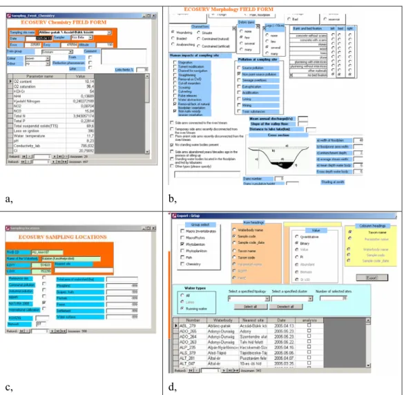
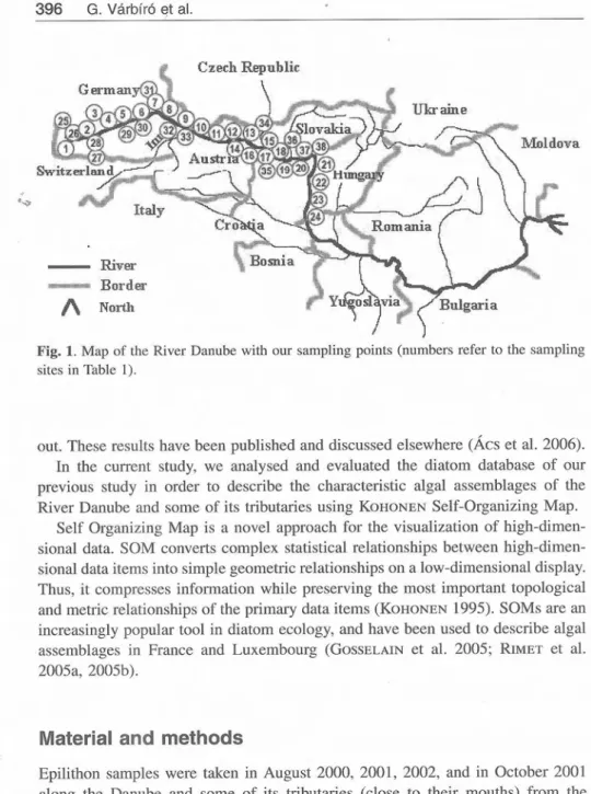
Neural networks in ecology. 18. provide a nation-wide overview of the ecological status of the water bodies. Sampling and assessment methods have been selected for all biological elements including fish, macrophyte, phytoplankton, phytobenton and macroinvertebrates. (Arcadis, 2005) The final database contains 70 tables and thousands of individual records. Some form of the database can be seen in Fig. 7.. a,. b,. c,. d,. Fig. 7. Selected forms from the ECOSURV database, a, Chemical sampling events form; b, hydromorphological information; c, Sampling locations form; d, Data export form..

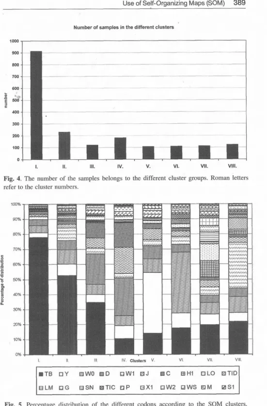
Neural networks in ecology. 19. Results “although our results are in contradiction with the hypotheses and statistically not significant, but from the figures its clearly visible …”. Paper 1. The phytoplankton database of the Middle Danube Basin was analysed and evaluated in order to describe the characteristics algal assemblages of the rivers. The dataset were extracted from the database of the Hungarian monitoring network and academic institutions. The database which has been included in the analysis contains the results of 1897 phytoplankton investigation from 189 locations. Implementing the SOM method we can identify the different algal communities which characterise different river types.. I. 100% 90%. Percentage of distribution. 80%. II. III. VIII.. 70% 60% 50% 40% 30% 20% 10% 0%. VI.. I.. III.. IV.. V.. VI.. VII.. VIII.. Clusters. IV.. VII.. II.. V.. Fig. 8. Clusters of the SOM based on codon abundances. TIB. Y. W0. D. W1. J. C. H1. LO. TID. LM. G. SN. TIC. P. X1. W2. WS. M. S1. Fig. 9. The distribution of the different codons according to the SOM clusters, in percentage of the total biomass..

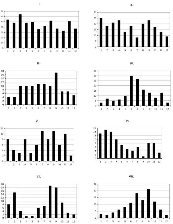
Neural networks in ecology. 20. I.. II.. 70. 30. 60. 25. 50. 20 40. 15 30. 10 20. 5. 10. 0. 0 1. 2. 3. 4. 5. 6. 7. 8. 9. 10. 11. 1. 12. 2. 3. 4. 5. 6. III.. 7. 8. 9. 10. 11. 7. 8. 9. 10. 11. 8. 9. 10. 8. 9. 12. IV.. 18 16 14. 35 30 25. 12 10 8 6. 20 15 10. 4 2 0. 5 0. 1. 2. 3. 4. 5. 6. 7. 8. 9. 10. 11. 12. 1. 2. 3. 4. 5. 6. 12. VI.. V. 16. 12. 14. 10. 12. 8. 10 8. 6. 6 4. 4. 2. 2 0. 0. 1 1. 2. 3. 4. 5. 6. 7. 8. 9. 10. 11. 2. 3. 4. 5. 6. 7. 11. 12. 12. VIII.. VII. 25. 20 18 16 14 12 10 8 6 4 2 0. 20 15 10 5 0. 1. 2. 3. 4. 5. 6. 7. 8. 9. 10. 11. 12. 1. 2. 3. 4. 5. 6. 7. 10. 11. 12. Fig. 10. Seasonal distribution of the selected clusters. Roman letters means the cluster numbers, vertical axis represents the months, while horizontal axis the number of samples belonging to that given month..

Neural networks in ecology. 21. The algal communities were described as different ratios of algal functional groups. Since some of the groups are in close relation with certain types of environmental pressure it is also possible to highlight those rivers or river sections (or those periods) which are far from the expected good ecological status. We identified eight clusters or river types. (Fig. 8.) Type I. This is the most frequent phytoplankton type which is representative for the upper section of rivers. The dominant codon is the TB (bentic diatoms) with more than 70 % of the total biomass abundance (Fig. 9.). This association has no seasonal preference. The most frequent taxa are Nitzschia palea, Nitzschia fonticola, Navicula capitatoradiata, Surirella brebissonii, Diatoma vulgaris. Type II. Members of the TB group are dominating type I1 (Fig. 9.) but the elements of the Wo and W1 functional groups (Chlamydomonas reinhardtii, Euglena spp.) indicate organic pollution. This type is also characteristic for upstream sections of rivers. Only a slight seasonal preference for early spring and autumn can be found. Type III. This is typical plankton of small rivers with the dominance of TB and D (Fig. 9.) codons. This assemblage occurs on those river sections where the retention time due to hydro-morphological changes or upper stream reservoirs enables real phytoplankton to develop. Type IV. This association can be referred to as "Danube type" summer plankton. The most important codons are D, J and C (Fig. 9.). Dominant species of this association are Stephanodiscus hantzschii, Cyclotella comta Skeletonema potamos and Nitzschia acicularis from codon D, Cyclotella meneghiniana from codon C, and Scenedesmus species from codon J. However, the favourable season of this type is the early summer (Fig. 10). Certain species such as Stephanodiscus invisitatus could bloom however, in the Danube during winter (Kiss and Genkal, 1993)..

Neural networks in ecology. 22. Type V. This type could be mainly found on the lower section of the river Tisza with the dominance of Y codon (Fig. 9.). Cryptomonas reflexa, C. marssonii, C. rostratiformis, Rhodomonas minuta become dominant in this section. Development of this association is absolutely independent from the seasons. (Fig. 10.) Type VI. The characteristic functional group of type VI is Wo (Fig. 9.). The dominance of this group is due to very strong organic pollution. Chlamydomonas spp., Euglena viridis, Polytoma uvella, Spermatozopsis exultans are typical elements of this assemblage. This type of plankton is usually dominant in winter and early spring (Fig. 10.) Type VII. This type is a mixture of a very divers association with the presence of relatively rare groups like Lo, HI, L,, S, (Fig. 9.). The occurrence of this type is expected in slow flowing channels and small rivulets in late winter and summer. The bimodal character of the type VII is cause by the Lo functional group. This plankton type frequently occurs in the summer epilimnion of lakes (Reynolds et al., 2002). Several dinophytes, however, can be important members of the winter phytoplankton (Grigorszky et al., 1998). Therefore it would be necessary to separate certain oligotherm Peridinium tax Type VIII. The dominant codon of this type is the W1 (Fig. 9.) which is according to Reynolds characteristic for small organic pools. Frequent taxa are the metaphytic Phacus and Trachelomonas spp. This type is typical in slow-flowing rivulets and channels which are under the risk of organic pollution and have rich macrophyte vegetation. Development of this type is expected in summer..

Neural networks in ecology. 23. Paper 2. In this paper the investigation of the benthic diatom flora of the River Danube is presented. The investigations include samples from the source streams to the end of the Hungarian stretch during a three years period. Characteristic diatom assemblages were established using SOM algorithm. K-means clustering of the SOM allocated 5 different sample groups (clusters) (Fig. 11a). With few exemptions, the first, second and third clusters fell in the GermanAustrian stretch, whereas the fourth and fifth clusters fell in the SlovakianHungarian stretch. Temporal differences were less pronounced: the five clusters were mainly organized by the sampling localities. The first cluster was formed by some sampling points scattered along the German and Austrian stretches, including the tributaries Enns and Lech. The second cluster comprised the sampling points around the source of the Danube such as the Breg and Brigach sources and streams, the first stretch of the River Danube after the fusion of Breg and Brigach, furthermore the tributaries Ipel, Morava and Garam. The third cluster was formed by the sampling sites on the lower part of the Austrian stretch. The fourth cluster was mostly built up by Slovakian, and the fifth by the Hungarian sampling sites, although the clustering is not perfectly unambiguous. The character species of the five sample clusters were defined (Fig.11a.). We found that the clusters 1 and 2 were characterized by Achnanthidium minutisimum (AMIN), Denticula tenuis (DTEN), Nitzschia fonticola (NFON), Psammothidium bioretii (ABIO), Melosira varians (MVAR), Planothidium subatomoides (ASAT). The character species of cluster 3 is Amphora pediculus. (APED), while character species of the clusters 4 and 5 are Nitzschia dissipata (NDIS), Navicula cryptotenella (NCTE), Cocconeis placentula var. euglypta (CPLA), Rhoicosphenia abbreviata (RABB), Nitzschia inconspicua (NINC)(Fig. 11b.). However, not all of these species had equally high SI values. Thirteen species had higher SI values, these were Amphora pediculus, Achanthidium minutissimum, Cocconeis placentula.

Neural networks in ecology. 24. var. euglypta, Nitzschia inconspicua, N. dissipata, Denticula tenuis, Rhoicosphenia abbreviata, Navicula tripunctata (NTPT), Navicula cryptotenella (NCTE), Staurosirella pinnata (FPIN), Nitzschia fonticola (NFON), Melosira varians and Nitzschia amphibia (NAMP). Considering the average relative abundance values of the character species of the five cluster groups it is obvious that the main difference between the cluster groups is not so much the species composition, but rather the different relative abundance ratios of the different species in the different clusters. This arrangement is also well in agreement with the poorer water quality of the lower, and the better water quality of the upper stretch. AMIN. 0.537. APED. 0.248. 5. 0.0135. NDIS. 0.0255. NINC. 0.0676. 0.00567. 0.00445. d. d. DTEN. 1 2. 0.0149 d. 0.135. 0.055. 4. 0.127. d. 0.107. 0.251. 0.223. d. 3. CPLA. 0.458. FPIN. MVAR. 0.131. 0.0509. 0.0563. 0.0635. 0.0265. 0.0281. 0.000171. 0.00261. d. 0.000597. d. NAMP. d. NCTE. NFON. 0.0634. 0.0776. 0.0798. 0.0319. 0.046. 0.0453. 0.00132. 0.0153. d. d. NTPT. 0.0118 d. RABB. a,. 0.077. 0.0952. 0.0418. 0.0494. 0.00774. 0.00555. d. d. b, Fig. 11. a, Clusters of the sampling site by K-means clustering of the SOM. b, Individual SOM maps of the characteristic species. Scale bars showing the species calculated abundances by the learning process of the SOM in percentage. Abbreviations of the species can be found in the text..

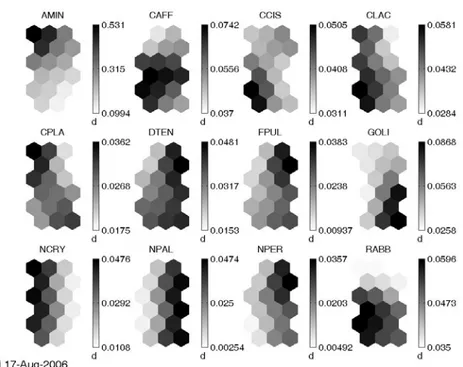
Neural networks in ecology. 25. Paper 3. The periphyton of the Lake Velencei which is a diverse and dense community were investigated in this article. The main interest was to distinguish the differences of periphyton communities according to the different substrate type. More than 120 algal species were found in this study, most of them are diatoms. According to the SOM analysis based on algological data (species composition and their abundance), samples of different substrata formed two distinctive groups. Old reed (OR), andesite (A) and granite (G) were grouped together, respectively, and polycarbonate (PC) and green reed (GR) clearly separated from the other three in May (Fig. 12.). Achnanthidium minutissimum and Navicula cryptotenella, a pioneer colonist diatom species were found to be vigorously dominant on all substrata. In November, based on the SOM analysis, granite and andesite come together with green and old reeds comprised one group, plexi and polycarbonate the other. These similarity was due to the presence of A. minutissimum, strongly. dominating. polycarbonate. both. substrata.. plexi. and. Characteristic. species were also Fragilaria pulchella and Nitzschia. perminuta. for. this. type. of. substrates, while for green and old reed a clear gradient of increasing of Nitzshia palea and Gomphonema olivaceum var. olivaceum can be viewed from the SOM component planes. (Fig. 13.) Fig. 12. Clustered SOM based on species composition, the last letter means the month(may=M, November=N) The first letter represents the substrate (old reed=OR, green reed=GR, granite=G, andezi t=A, polycarbonate=PC).

Neural networks in ecology. 26. Fig. 13. The component planes of the SOM, the vertical bars represent species abundances in percentage. Achnanthidium minutisimum (AMIN), Cymbella affinis var. affinis (CAFF), Cymbella cistula (CCIS), Cymbella lacustris (CLAC), Cocconeis placentula var. euglypta (CPLA), Denticula tenuis (DTEN), Fragilaria pulchella (FPUL), Gomphonema olivaceum var. olivaceum (GOLI), Navicula cryptocephala (NCRY), Nitzschia palea (NPAL), Navicula permitis (NPER), Rhoicosphenia abbreviate (RABB).. Paper 4. Monitoring of the naturally occurring algal communities in rivers provide data on species composition, species number, diversity, or quantitative occurrence of the algae. Experts of administrative institutions who are responsible for water quality management need simple numerical values rather than species lists or scientific evaluation of the assemblages. Since up to now, little attention has been attended to the application of the phytoplankton for evaluation of ecological state of the rivers, the present study aims to show a new assessment method. The method is.

Neural networks in ecology. 27. based on the functional group of algae, described for lakes by Reynolds (Reynolds , 2002), represented in the potamoplankton and provides a single index number (Q). The index has been tested on phytoplankton data of different rivers, and proved to be more sensitive than the earlier used saprobic index. To achieve an index, each species in the sample must be assigned to the appropriate functional group. Then the relative share of each functional groups are calculated. Relative shares are then multiplied by the factor number. The sum of these scores is the index. The reference values of the upper river sections are close to 5, while those of the lower river stretches are approximately 4. The method has been tested with hundreds of phytoplankton samples, it is simple, and after applying to a phytoplankton database can be computerised easily. The new assessment method has been tested by using different datasets from Hungarian rivers that contain phytoplankton data against the Pantle-Buck index (Pantle & Buck, 1955), which is the officially accepted qualification method in Hungary and several other countries in Europe.. Paper 5. In this study the results of the first nation wide survey of benthic river diatoms is presented. The dataset is robust as the primary sources of uncertainty in diatom training sets (choice of site and substrate for sampling, inter-operator differences in diatom taxonomy and counting techniques (Besse-Lototska et al., 2006) were eliminated as much as possible. Moreover, parallel with the diatoms, investigations were made on other biological quality elements, including macro-invertebrates and fish. In total, nearly 500 taxa were found in the 339 sites. This certainly does not include all diatom taxa in the inland waters of a country like Hungary, which probably has number between 1000 and 2000 'conservative' taxa. The present study provided a relatively homogeneous diatom data set for the whole country, which is lacking in most of the other European countries..

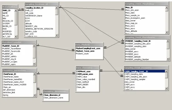
Neural networks in ecology. 28. Many of the diatom taxa were very rare and occurred only in one or in a few samples. The commonest genera are Navicula (104 taxa), followed by Nitzsclzia (go), Fragilaria (43), Achnanthes (41), Gomphonema (30) and Cymbella (26). The most common taxa are listed in Table 2. The most common species, Achnanthidium minutisimum, is also the most common freshwater diatom species in the world. The majority of the other common taxa are characteristic of eutrophic, alkaline waters. Some of these are tolerant to organic pollution (e. g. Gomphonema parvulum, Nitzschia paleacea), others require cleaner waters (e. g. Achnanthes biasolettiana, Gomphonema micropus). Meridion circulare is one of the very few diatom species which are characteristic for running waters (Van Dam et al., 1994). Species from acidic or oligotrophic waters are rare in the dataset: the most common one is Eunotia bilunaris. The study shows that despite the intensive human use of over 90 % of the area of the country, natural variation is still the predominant factor responsible for the composition of river diatom assemblages. The diatom database used in the paper was part of the ECOSURV database. The author of the theses was responsible for building the database structure as well as providing the relevant data matrixes. The structure and the connection between the tables involved in the analysis can be seen in Fig. 14..

Neural networks in ecology. 29. Fig. 14. The table structure of the diatom database used in the analysis in Paper 5. The variables on the left side considered as static whereas on the rights side the dynamic variables can be seen. A better understanding of the relationships between diatom assemblages and environmental factors (including stressors) will be gained by a more time-intensive monitoring of selected stations in the present network..

Neural networks in ecology. 30. Summary The need for better techniques, tools and practices to analyse ecological systems within an integrated framework at wider scales has never been so great. The biological monitoring of the water currents in Hungary provided large volume datasets during the last years thanks to the EU Water Framework Directive (2000). For easy handling the data of the monitoring it is essential to store them in an appropriate ecological database. This database should be capable of the storage of relevant static and dynamic variables from the ecosystems and should also allow the production of matrix inputs for ecosystem analysis. In case of large volume of data, the traditional multivariate statistical methods like cluster analysis and ordination are difficult to interpret and present the information. Self Organizing Map is a novel approach for the visualization of high-dimensional data. In the theses I described in details the SOM algorithm as well as the basic structure of an ecological database. By combining the database structures and the SOM algorithm we were able to characterize frequent Hungarian running water types according to their characteristic phytoplankton assemblages. I constructed the phytoplankton and phytobenton database which is presently in use in the environmental authorities, and is concerned as National Database. By the application of SOM methods we characterized the upper Danube section based on their characteristic diatom communities, and described the differences and similarities of the periphyton of the Lake Velencei on different substrates..

Neural networks in ecology. 31. Összefoglalás A doktori értekezés előzményei és célkitűzései; A 2001-ben bevezettet EU Vizkeretirányelv, melynek célja a felszíni és felszín alatti vizek jó ökológiai állapotának elérése 2015-re, több élőlénycsoport rendszeres monitorozását irja elő, mely tevékenység nagy mennyiségű ökológiai adatot eredményez. A rendszeres adatgyűjtés és az így keletkező adatok adatbázisba rendezése nemcsak a strukturált adatfeldolgozást teszi lehetővé, hanem az adatok kiértékelésében is nagy szerepet kap. A benne tárolt adatok élettartama nemcsak a vizsgálat idejére korlátozódik, így azok a későbbi elemzésekben is részt vehetnek. Az ökológiai folyamatok tér és időbeli összetettsége, a fajok és a környezeti változók közötti nem lineáris kapcsolat és a változók normalitásának hiánya komoly kihívást jelent az adatfeldolgozásban és az ökológiai folyamatok feltárásában. A mesterséges neurális hálózatok vonzó alternatív eszközzzé váltak az ökológiai adatelemzés során, mert számos előnyös tulajdonsággal rendelkeznek, mint például a nem-linearitás, adaptivitás, általánosítás és modell függetlenség (nem szükséges apriori modell). A neurális hálózatok alkalmazása, - bár már az 1950-s években megtörténtek a kezdeti lépések - csak az utóbbi évtizedekben terjedt el és vált az ökológusok által is használt statisztikai eszköztár részévé. A neurális hálózatok erős és hathatós segítséget nyújtottak az ökológiai modellezésben, osztályozási feladatok megoldásában és a mintázatelemzések során (Paisley et al., 2003). A neurális hálózatokat számos hidrológiai és hidrobiológiai kutatásban sikerrel alkalmazták; így például a vízminőségi paraméterek modellezésében (e.g. Daniell and Wundke, 1993; Lachtermacher and Fuller, 1994; Schizas et al., 1994; Kaluli et al., 1998; Wen and Lee, 1998) vagy az élőlényközösségek és a környezeti változók.

Neural networks in ecology. 32. közötti összefüggések vizsgálatában (e.g. Chon et al., 1996; Lek et al., 1996; Recknagel et al., 1998; Guegan et al., 1998; Lee et al., 1998; Maier et al., 1998). Nagymennyiségű adat elemzésénél a hagyományos többváltozós elemzések számos esetben nehezen értelmezhetők és eredményik nem jeleníthetők meg közérthető formában. A Kohonen-féle Önszervező Térkép Módszer egy olyan neurális hálózati típus, amely lehetővé teszi nagymennyiségű, összetett, (több dimenziós), adatok elemzését és értékelését. A Teuvo Kohonen által kifejlesztett módszer a dimenzió csökkentése révén a kiindulási adatmátrixot kétdimenziós hexagonális térképre képezi le, megőrizve a kiindulási adatok topológiai és metrikai sajátságait (Kohonen 2001). A módszer legfőbb erénye az adatok szemléletes megjelenítése (Vesanto and Alhoniemi 2000). Anyag és módszer A statisztikai elemzések elvégzéséhez az önszervező térkép (SOM) algoritmust használtuk. Az algoritmus lehetővé teszi nagy adatbázisok sokdimenziós adatainak leképezését kétdimenziós hexagonális térképpé. Az egymáshoz közeli térkép egységek (neuronok) úgy helyezkednek el a végső térképen, hogy az egymáshoz hasonló tulajdonsággal rendelkező neuronok egymás közelében, míg a különbözőek a térkép távolabbi pontjain helyezkednek el. A SOM a mintákat és a változókat egyidejüleg is képes megjeleníteni, s ugyanakkor a változók fontosságát is meghatározhatjuk. (Kohonen, 2001). Az értékelés során a SOM Toolbox modult (http://www.cis.hut.fi/projects/somtoolbox) és a MATLAB™ fejlesztői környezetet használtuk. A SOM neurális hálózat a nem-ellenőrzött tanulási típusú hálozatok kategóriájába tartozik, ami azt jelenti, hogy nem adunk meg kimeneti paramétert, a csoportok képzését az algoritmus önnállóan végzi. Maga a hálózat egy bemeneti (input) és egy kimeneti (output) rétegből áll. A bemeneti réteg.

Neural networks in ecology. 33. tartalmazza a mintaegységeket (SU), a kimeneti réteg a virtuális egységekből (VU) vagy neuronokból áll. A kimeneti réteg neuronjai a bemeneti réteg súlyvektorainak megfelelő mintázatot vesznek fel egy tanulási folyamat során. Ez. ökológiai. analógiára. lefordítva. annyit. tesz,. hogy. a. kiindulási. mintavételekhez (SU) tartozó faj-abundancia viszonyokra jellemző lesz a végső SOM térkép neuronjainak súlyfaktora, azaz minden egyes neuron egy egy virtuális faj abundancia listával fog rendelkezni. Az eljárás kellően robosztus, lehetővé teszi több ezer mintavételi egység sűrítését néhány virtuális neuronba. A végső SOM térkép leggyakoribb ábrázolási módja a hexagonális rács (Fig. 2.). A SOM algoritmusát az alábbik szerint adhatjuk meg: •. 1. lépés: Ciklus t=0, a virtuális egységet (VUp) inicializáljuk, a súlyokat (w) az input adatokból töltjük fel.. •. 2. lépés: Egy mintaegységet kiválasztunk (SUj) véletlenszerűen. •. 3. lépés: Egy megfelelő metrika segítségével meghatározzuk a SUj és az összes VUp közötti távolságot.. •. 4. lépés: A SUj-hez legközelebbi VUc lesz a győztes neuron, ez a neuront Legjobban hasonlító egységnek (BMU) nevezzük. •. 5. lépés: A virtuális egységek VUp súlyfaktorai a tanulási szabály alapján módosulnak, úgy, hogy az új faktorok a SUj bemeneti vektorához hasonlítsanak.. •. 6. lépés: Újabb ciklus kezdődik t+1, amíg t <tmax addig 2. lépésre lép; a ciklus akkor fejeződik be, ha eléri a kívánt számú ismétlést .. Az első lépésben a felhasználó dönti el a térkép méretét. A kimeneti réteg neuronjainak oiptimális száma az alábbiak szerint számolható (Vesanto, 2000). Nn = 5 SU d Ahol Nn a neuronok száma a végső térképen és SUd a mintavételi egységek száma. A 3. lépésben a leggyakrabban használt távolság metrika az Euklideszi..

Neural networks in ecology. 34. Az 5. lépésben Euklideszi tanulási szabály hck(t) változója a szomszédsági függvény. A 4. lépésben kiválasztott BMU neuron nem az egyetlen, amelynek vektorait módosítjuk, hanem a szomszédos neuronok is módosulnak. A leggyakrabban használt szomszédsági függvény a Gauss féle: ⎛ rk − rc 2 hck (t ) = α (t ) ⋅ exp⎜ − ⎜ 2σ 2 (t ) ⎝. ⎞ ⎟ ⎟ ⎠. ||rk – rc ||: az Euklideszi távolság a győztes neuron VUc és a térkép többi neuronja VUk.között, σ: időben csökkenő faktor azt határozza meg, hogy a térkép mekkora része érintett a tanulási folyamatban, α: a tanulási faktor. Mindkét faktor idővel csökken, és nullához konvergál. A SOM jellemzésére és a karakterfaj elemzések során a strukturális indexet (SI) használtuk. Az index azt mutatja meg, hogy az egyes változók (súlyfaktorok) milyen mérétékben felelősek a SOM térkép topológiájáért (Park et al., 2005). Azok a változók (esetünkben fajok) amelyek nagyon erős grádiens eloszlást mutatnak, nagy SI index értékkel rendelkeznek, karakterfajoknak tekinthetők. Az SI értékét az alábbiak szerint számolhatjuk: S. j −1. SI i = ∑∑ j =1 k =1. Wij − Wik r j − rk. ahol wij és wik az ith faj súlyfaktorai, ||rj−rk|| a topológiai távolság a térkép két j és k neuronja között, S a SOM térkép neuronjainak száma. Az algoritmus eredményeképpen kapott térkép neuronjait a kiindulási mintaegységekkel megfeleltethetjük és ábrázolhatjuk. Bár az egymáshoz hasonló minták egymás közelében helyezkeden el, a mintacsoportok elkülönítése nem minden esetben egyértelmű. A mintacsoportok elkülönítésére számos lehetőségünk van. Használhatunk hagyományos klaszterezési technikát. Mi az elemzések során a szakirodalom által.

Neural networks in ecology. 35. ajánlott k-átlag módszert használtuk. A megfelelő clusterszám meghatározása a Davies-Bouldin indexet felhasználásával történt (Davies and Bouldin, 1979) Az ökológiai adatbázis az adatok illetve rekordok stukturált összessége. Napjainkban a leggyakrabban használt adatbázis modell a relációs adatmodell. A reláció nem más, mint egy táblázat, a táblázat soraiban tárolt adatokkal együtt. A relációs adatbázis, pedig a relációk összessége. Ennek alapstruktúrája az adattábla, amely sorokból (rekordok) és oszlopokból (mezők) áll. A relációk vagy kapcsolatok az adatbázis táblái között állnak fenn. A táblák oszlopai vagy mezői az adatok tulajdonságai, pl. mintavételi hely neve, mintavétel dátuma, a sorok vagy adatok pedig a konkrét értékeket taralmazzák pl. 2009.05.27., Concó, Ács A relációs adatbázis előnye, hogy minimalizálja a tárolt redundáns információt, ezáltal csökkenti az adatbázis méretét és az egyszerre kezelt adatok mennyiségét, valamint a kapcsolatok révén bármely mező szerinti lekérdezét ill. csoportosítást lehetővé tesz.. Eredmények A disszetáció öt tudományos közleményt tartalmaz. A disszertációban részletesen bemutattam a SOM algoritmusát, valamint az ökológiai adatbázis szerkezetét. A megfelelő adatszerkezet és a SOM statisztikai módszer segítségével lehetővé vált magyarországi folyóvíz típusok jellemzése a fitoplakton közösségek alapján. Létrehoztam egy fitoplakton és egy fitobenton adatbázist amelyet jelenleg is használnak a Környezetvéfelmi Felügyelőségek és ezek részei az országos monitoring hálózatnak is..

Neural networks in ecology. 36. A SOM módszer segítségével jellemeztem a felső Duna szakasz diatóma közösségeit és a Velencei tavi, különböző aljzaton előforduló perifitonjának sajátosságait. Folyóvízi fitoplankton közösségek Use of Self-Organizing Maps (SOM) for characterisation of riverine phytoplankton associations in Hungary, (Várbíró et al., 2007) 1. A célkitűzésünk az volt, hogy a magyarországi folyóvizek jellemző fitoplakton közösségeit a meghatározzuk és jellemezzük. Az adatsor a magyarországi monitoring hálózat adatait tartalmazta és ezen adatok adatbázisba történő rendezése után vált értékelhetővé. Az elemzésben használt adatbázis 1897 mintavétel adatait tartalmazta 189 mintavételi hely esetében. A SOM módszer segítségével nyolc folyóvíztípust lehetett elkülöníteni. Minden típusra meghatároztuk a domináns fitoplakton közösséget és jellemeztük az egyes csoportokat. A fitoplakton taxonokat a Reynolds féle kodonbesorolás alapján elemeztük (Reynolds, 2002). Néhány csoport szoros összefüggést. mutatott. a. környezeti. változókkal. és. lehetővé. vált. azon. folyószakaszok illetve fitoplakton közösségek meghatározása, amelyek nem megfelelő ökológiai állapotot jeleznek. Az általunk meghatározott folyóvízi fitoplankton típusok (2. ábra): I. típus A folyók felső szakaszaira legjellemzőbb típus a TIB kodon (bentikus kovaalgák), gyakran 100% abundanciaértékkel. Leggyakoribb taxonok a Nitzschia palea, Nitzschia fonticola, Navicula capitatoradiata, Surirella brebissonii, Diatoma vulgaris. II. típus Ebben a típusban is a TIB csoport dominál, de jelentős arányban jelen vannak a szerves szennyezésre utaló W0 és W1 funkcionális csoportok fajai (Chlamydomonas reinhardtii, Euglena spp.)..

Neural networks in ecology. 37. III. típus Ez a típus a kisebb folyókra jellemző, ahol a víz tartózkodási ideje, hidromorfológiai beavatkozások miatt megnő és lehetővé teszi valódi plankton kialakulását. Jellemző kodonok a TIB és a D csoportok. IV. típus Ez a típus a Dunára jellemző plaktontípus. Jellemző kodonok a D, J és a C. Domináns fajok a D kodonba tartozó Stephanodiscus hantzschii, Cyclotella comta Skeletonema potamos és Nitzschia acicularis, a C kodonba tartozó Cyclotella meneghiniana és a J kodonba tartozó Scenedesmus fajok. V. típus Ebbe a típusba a Tisza alsó szakasza tartozik. A domináns kodon az Y, jellemző fajok a Cryptomonas reflexa, C. marssonii, C. rostratiformis. VI. típus Ebbe a típusba a szerves szennyezéssel terhelt vizek tartoznak. A terhelést jellző W0 kodon dominál, jellemző fajok Chlamydomonas spp., Euglena spp., (Polytoma uvella, Spermatozopsis exultans.) VII. típus A lassú folyású kis csatornák és erek jellemző asszociációja. Több relatívan ritka kodon fordul elő benne, például L0, HI, L, S. Szezonálisan bimodalis eloszlás jellemzi, azaz a nyári és a téli vegetációs periódusban is dominánsá válhatnak a H1 másrészt az L0 (Dinofita) funkcionális csoportok fajai. VIII. típus A W1 kodon dominanciája jellemzi ezt a típust, amely Reynolds szerint a kis szerves tavak jellemző plantkonja. Gyakori taxonok a metafitikus Phacus és Trachelomonas fajok. Ez a típus a dús növényzettel benőtt csatornákra jellemző, tipikusan a nyári vegetációs periódusban előforduló asszociáció. A Duna bentikus kovaalga flórája Use of Kohonen Self Organizing Maps (SOM) for the characterisation of benthic diatom associations of the River Danube and its tributaries. (Várbíró et al., 2007) Ebben a cikkben a Duna felső szakasza, bentikus kovaalga flórájának bemutatása történt meg..

Neural networks in ecology. 38. A mintavételi helyek a Duna forrásától a Magyarországi szakaszának végig terjedtek és három éves periódust öleltek fel. A jellemző kovaalga közösségeket SOM módszer segítségével határoztuk meg. Az elkészült SOM térképet k-átlag klaszterezési eljárással 5 klaszterre különítettük el. Néhány kivételtől eltekitve az első három klasztercsoportba a Német-Osztrák Duna-szakasz került, a 4. és 5. csoportok a Szlovák-Magyar szakaszra estek. A mintavételek időbeni különbsége nem volt számottevő. A klaszterek a mintavételi helyek szerint alakultak ki. Az 1-2. klaszter karakterfajai, melyet a strukturális index segítségével határoztunk meg: Achnanthidium minutisimum, Denticula tenuis, Nitzschia fonticola, Psammothidium bioretii, Melosira varians, Planothidium subatomoides. A 3. klaszter karakterfaja az Amphora pediculus, míg a 4-5. klaszteré a Nitzschia dissipata, Navicula cryptotenella; Cocconeis placentula var. euglypta, Rhoicosphenia abbreviata, Nitzschia inconspicua voltak. Aljzat szerepe kovaalga közösségek kialakulásában Comparative algological and bacteriological examinations on biofilms developed on different substrata in a shallow soda lake (Ács et al.,2008) A felmérés a Velencei tó gazdag perifiton közössének vizgálatára irányult. Arra a kérdésre kerestük a választ, hogy meghatározzuk az eltérű aljzatokon előforduló kovalaga közösségek összetételét. A SOM analízis alapján a kovalga közzösségek abundancia viszonyai a májusi mintavételek esetén két csoportra különíthetők el. Az avas nád, az andezit és a gránit aljzatok alkottak egy csoportot, a zöld nád és a polikarbonát pedig egy másikat. Az Achnanthidium minutissimum és Navicula cryptotenella, mint pionír kovaalga kolonista fajok, erőteljesen meghatározók voltak valamennyi aljzat esetén. Novemberben a SOM analízis alapján az avas és a zöld nád az andezit és gránit aljzatal alkotott egy csoportot, míg a polikarnonát a plexi aljzattal. Ez a hasonlósága az Achnanthidium minutissimum, fajnak volt köszönhető, ami az utóbbi két.