Two Reflected Gray Code based orders on some restricted growth sequences

arXiv:1306.5464v1 [math.CO] 23 Jun 2013

Two Reflected Gray Code based orders

on some restricted growth sequences

Ahmad Sabri _Vincent Vajnovszki

LE2I, Universit´e de Bourgogne LE2I, Universit´e de Bourgogne BP 47870, 21078 Dijon Cedex, France BP 47870, 21078 Dijon Cedex, France

ahmad.sabri@u-bourgogne.fr vvajnov@u-bourgogne.fr

Dept. of Informatics, Gunadarma University Depok 16424, Indonesia

sabri@staff.gunadarma.ac.id

June 25, 2013

Abstract

We consider two order relations: that induced by the m-ary reflected Gray code and a suffix partitioned variation of it. We show that both of them when applied to some sets of restricted growth sequences still yield Gray codes. These sets of sequences are: subexcedant or ascent sequences, restricted growth functions, and staircase words. In each case we give efficient exhaustive generating algorithms and compare the obtained results.

1

Introduction and motivations

The term ‘Gray code’ was taken from Frank Gray, who patented Binary Reflected Gray Code (BRGC) in 1953 [1]. The concept of BRGC is extended to Reflected Gray Code (RGC), to accommodate m-tuples (sequence), with m > 2 [2]. In these Gray codes, successive sequence differ in a single position, and by +1 or−1 in this position. More generally, if a list of sequences is such that the Hamming distance between successive sequences is upper bounded by a constant d, then the list is said a d-Gray code. So in particular, BRGC and RGC are 1-Gray codes. In addition, if the positions where the successive sequences differ are adjacent, then we say that the list is a d-adjacentGray code.

2

Preliminaries

2.1 Gray code orders

LetGn(m) be the set of lengthn m-ary sequencess1s2. . . snwithsi ∈ {0,1, . . . , m−1}; clearly, Gn(m) is the product set{0,1, . . . , m−1}n. TheReflected Gray Code (RGC for short) for the set Gn(m), denoted by Gn(m), is the natural extension of the Binary Reflected Gray Code to this set. The list Gn(m) is defined recursively by the following relation [2]:

Gn(m) =

ǫ if n= 0,

0Gn−1(m), 1Gn−1(m), 2Gn−1(m), . . . , (m−1)G_n′₋1(m) if n >0,

(1)

whereǫ is the empty sequence, Gn−1(m) is the reverse of Gn−1(m), andG_n′₋1(m) is Gn−1(m) or

Gn−1(m) according to m is odd or even.

InGn(m), two successive sequences differ in a single position and by +1 or−1 in this position. A list for a set of sequences induces an order relation to this set, and we give two order relations induced by the RGC and its variation, namely RGC order [10] and Co-RGC order.

We adopt the convention that lower case bold letters represent tuples, for example: s ₌

s1s2. . . sn,a=a1a2. . . ak,b=bk+1bk+2. . . bn.

Definition 1. The Reflected Gray Code order ≺on Gn(m) is defined as: s_{=s1s2. . . sn is less}

thant_{=t1t2. . . tn, denoted by}s_≺t_{, if either}

• Pk−1

i=1 si is even and sk< tk, or

• Pk−1

i=1 si is odd and sk> tk,

wherek is the leftmost position wheres _andt _differ.

It is easy to see thatGn(m) defined in relation (1) lists sequences in Gn(m) in ≺order. Now we give a variation of Gn(m). Lets1s2. . . snbe a sequence inGn(m). The complement of si, 1≤i≤n, is

(m−1−si),

and the reverse ofs1s2. . . sn is

snsn−1. . . s1.

LetGen(m) be the list obtained by transforming each sequences inGn(m) as follows:

• complementing each digit ins_{if m is even, or complementing only digits in odd positions}

if m is odd, then

• reversing the obtained sequence.

Clearly,Gen(m) is also a Gray code forGn(m), and the sequences therein are listed in Co-Reflected Gray Code order, as defined formally below.

Definition 2. The Co-Reflected Gray Code order≺c on Gn(m) is defined as:

s_{=s1s2. . . sn is less than} t_{=t1t2. . . tn, denoted by}s_≺ct_{, if either}

• Pn_i=k+1si+ (n−k) is odd andsk< tk,

wherek is the rightmost position wheres _andt_differ.

Although this definition sounds somewhat arbitrary, as we will see in Section 4, it turns out that ≺c order gives suffix partitioned Gray codes for some sets of restricted growth sequences. Obviously, the restriction of Gn(m) (resp. Gen(m)) to a set of sequences is simply the list of sequences in the set listed in ≺(resp. ≺c) order.

2.2 Restricted growth sequences defined by means of statistics

Through this paper we consider sequences over non-negative integers. A statistic on a set of sequences is an association of an integer to each sequence in the set. For a sequence s1s2. . . sn,

its length minus one, numbers of ascents/levels/descents, maximal value, and last value are classical examples of statistics. They are defined as follows, see also [14]:

• len_(s1s2. . . sn) =n−1;

• asc_{(s1s2. . . sn) = card{i|1≤i < n andsi < si+1};}

• lev_{(s1s2. . . sn) = card{i|1≤i < n and si=si+1};}

• des_{(s1s2. . . sn) = card{i|1≤i < n and si> si+1};}

• m_(s1s2. . . sn) = max{s1, s2, . . . , sn};

• lv_{(s1s2. . . sn) =sn.}

Ifst _{is one of the statistics} len_,asc_,m_{, and} lv_{, then} st_{satisfy the following:}

st_(s1s2. . . sn)≤n−1, (2)

and

if sn=st_(s1s2. . . sn₋1) + 1,thensn=st(s1s2. . . sn₋1sn). (3)

On the contrary, the statistics lev_and des_{do not satisfy relation (3). Accordingly, through this} paper we will consider only the four statistics above. However, as we will point out, some of the results presented here are also true for arbitrary statistics satisfying relations (2) and (3).

Definition 3. For a given statistic st_{, an} st_{-restricted growth sequence s1s2. . . sn is a sequence} withs1 = 0 and

0≤sk+1 ≤st(s1s2. . . sk) + 1 for 1≤k < n, (4)

and the set of st_{-restricted growth sequences is the set of all sequences s1s2. . . sn satisfying} relation (4).

From this definition, it follows that any prefix of an st_{-restricted growth sequence is also (a} shorter)st_{-restricted growth sequence.}

Remark 1. Ifst _{is a statistic satisfying relations (2) and (3) above, then}

2. if s1s2. . . sn is an st-restricted growth sequence, then for any k, 1 ≤ k < n, sk+1 =

st_{(s1s2. . . sk) + 1 impliessk+1 =}st_{(s1s2. . . sksk+1).}

The sets of st_{-restricted growth sequences, where} st _{is one of the statistics} len_,asc_,m_{, and} lv_{, are defined below.}

Definition 4.

• The setSEn of subexcedant sequencesof length nis defined as:

SEn={s1s2. . . sn|s1= 0 and 0≤sk+1≤len(s1s2. . . sk) + 1 for 1≤k < n};

• The setAn of ascent sequencesof length nis defined as:

An={s1s2. . . sn|s1 = 0 and 0≤sk+1 ≤asc(s1s2. . . sk) + 1 for 1≤k < n};

• The setRnof restricted growth functions of lengthn is defined as:

Rn={s1s2. . . sn|s1= 0 and 0≤sk+1≤m(s1s2. . . sk) + 1 for 1≤k < n};

• The setSn of staircase wordsof length nis defined as:

Sn={s1s2. . . sn|s1 = 0 and 0≤sk+1≤lv(s1s2. . . sk) + 1 for 1≤k < n}.

Notice that alternatively, SEn={0} × {0,1} ×. . .× {0,1, . . . , n−1}.

Remark 2. Sn⊂Rn⊂An⊂SEn⊂Gn(n).

Below we give examples to illustrate Remark 2.

Example 1.

• If s_{= 010145, then} s_{∈SE6, but}s_{∈/ A6,} s_{∈/ R6 and} s_{∈/ S6.}

• If s_{= 010103, then} s_∈SE6, s_{∈A6, but}s_{∈/ R6 and} s_{∈/ S6.}

• If s_{= 010102, then} s_∈SE6, s_{∈A6, and}s_{∈R6, but}s_{∈/ S6.}

• If s_{= 010101, then} s_∈SE6, s_∈A6, s_{∈R6 and}s_∈S6.

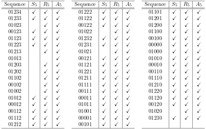
See Table 3 for the sets S5,R5, andA5 listed in≺order, and Table 4 for the same sets listed in

≺c order. We denote by

• Xnthe list for the set Xn in≺order, and by Xenthat in ≺c order;

• succX(s), s∈Xn, the successor of sin the setXn listed in≺order; that is, the smallest sequence in Xn larger than s_{with respect to≺ order;}

• succ_gX(s) the counterpart of succX(s) with respect to≺c order;

• first(L) the first sequence in the listL;

2.3 Constant Amortized Time algorithms and principle

An exhaustive generating algorithm is said to run in constant amortized time (CAT for short) if the total amount of computation is proportional to the number of generated objects. And so, a CAT algorithm can be considered an efficient algorithm.

Ruskey and van Baronaigien [15] introduced three CAT properties, and proved that if a recursive generating procedure satisfies them, then it runs in constant amortized time (see also [16]). They called this general technique to prove the efficiency of a generating algorithm asCAT principle, and the involved properties are:

1. Every call of the procedure results in the output of at least one object;

2. Excluding the computation done by the recursive calls, the amount of computation of any call is proportional to the degree of the call, that is, the number of call initiated by the current call;

3. The number of calls of degree one, if any, is O(N), where N is the number of generated objects.

All the generating algorithms we present in this paper satisfy these three desiderata, and so they are efficient.

3

The Reflected Gray Code order for the sets

SE

_n

_,

A

_n

_,

R

_n

_{, and}

S

_n

3.1 The bound of Hamming distance between successive sequences in the lists SEn, An, Rn, and Sn

Here we will show that the Hamming distance between two successive sequences in each of the mentioned lists is upper bounded by a constant, and so the lists are Gray codes.

Without another specification, Xn generically denotes one of the sets SEn, An,Rn, or Sn; and Xn denotes its corresponding list in ≺order, that is, one of the lists SEn, An, Rn, or Sn. Later in this section, Theorem 1 and Proposition 2 state that, in each case, the setXn listed in

≺order yields a Gray code.

Lemma 1. If s_{=s1s2. . . sn and}t_{=t1t2. . . tn are two sequences in Xn with} t_{= succX(}s_{) and}

k is the leftmost position where they differ, thensk=tk+ 1or sk=tk−1.

Proof. Let t_{= succX(}s_{) and kbe the leftmost position where they differ. Let us suppose that}

sk< tk and sk6=tk−1 (the case sk > tk and sk 6=tk+ 1 being similar). It is easy to check that

u_{=s1s2. . . sk}

−1(sk+ 1)0. . .0

belongs to Xn, and considering the definition of ≺ order relation, it follows that s _≺ u _≺ t_,

which is in contradiction witht_{= succX(}s_{), and the statement holds.}

If a _{=a1a2. . . ak ∈Xk, then for any n > k,} a _{is the prefix of at least one sequence in Xn,}

and we denote by a_{| Xn the sublist of Xn of all sequences having the prefix} a_{. Clearly, a list}

For a given a _{∈ Xk, the set of all x such that} a_{x ∈ Xk+1 is called the defining set of the}

prefix a_{, and obviously} a_{x is also a prefix of some sequences in Xn, for any n > k. We denote}

by

ωX(a_{) = max{x|}a_{x∈Xk+1} (5)}

the largest value in the defining set ofa_{. And if we denote ωX(}a_{) byM, then by Remark 1 we}

have

M = st₍a_{) + 1}

= st₍a_M).

And consequently,

ωX(a_{M) =} st₍a_{M) + 1}

= M + 1. (6)

The next proposition gives the pattern of s_{∈Xn, if} s_{= last(}a_{| Xn) or}s_{= first(}a_{| Xn).}

Proposition 1. Let k < n and a _{=a1a2. . . ak ∈Xk. If}s_{= last(}a_{| Xn), then the pattern of} s

is given by:

• if Pk_i=1ai is odd, then s=a0. . .0;

• if Pk_i=1ai is even and M is odd, then s=aM0. . .0;

• if Pk_i=1ai is even and M is even, then s=aM(M+ 1)0. . .0; where M denotes ωX(a).

Similar results hold for s _{= first(}a_{| Xn) by replacing ‘odd’ by ‘even’, and vice versa, for the}

parity of Pk_i=1ai.

Proof. Let s_{=a1a2. . . aksk+1. . . sn= last(}a_{| Xn).}

IfPk_i=1aiis odd, then by considering the definition of≺order, it follows thatsk+1is the smallest

value in the defining set ofa_{, and sosk+1= 0, and finally}s₌a_{0. . .0, and the first point holds.}

Now let us suppose thatPk_i=1ai is even. In this case sk+1 equals ωX(a) =M, the largest value

in the defining set of a_{. When in addition M is odd, so is the summation of} a_{M, the length}

k+ 1 prefix ofs_{, and thus}s₌a_{M0. . .0, and the second point holds.}

Finally, when M is even, then sk+2 is the largest value in the defining set of aM, which by

relation (6) is M+ 1. In this case M + 1 is odd, and thus s₌a_{M(M + 1)0. . .0, and the last}

point holds.

The proof for the cases_{= first(}a_{| Xn) is similar.}

By Proposition 1 above, we have the following:

Theorem 1. The lists An, Rn and Sn are 3-adjacent Gray codes.

Proof. Let Xn be one of the lists An, Rn or Sn, and t = succX(s). Let k be the leftmost position where s_and t _{differ, and let us denote by} a _{the length k prefix of}s_and a′ _{that of} t_;

so, s_{= last(}a_{| Xn) and} t_{= first(}a′_{| Xn). If k+ 3 ≤ n, then by Proposition 1, it follows that}

sk+3 =sk+4 =· · ·=sn= 0 and tk+3 =tk+4 =· · ·=tn = 0. So sand t differ only in position k, and possibly in positionk+ 1 and in positionk+ 2.

Now we show the adjacency, that is, if k+ 2 ≤ n and sk+1 = tk+1 implies sk+2 = tk+2. If sk+1=tk+1, by Lemma 1, it follows that the summation of the length kprefix of sand that of

• sk+1 =tk+1= 0, and by Proposition 1, it follows that sk+2=tk+2= 0; or

• sk+1 =tk+1 6= 0, and thussk+1 =tk+1 =ω(a) = ω(a′). In this case, ω(a) either is odd and

sosk+2=tk+2 = 0, or is even and sosk+2=tk+2 =ω(a) + 1.

In both cases, sk+2=tk+2.

It is well known that the restriction of Gn(m) defined in relation (1) to any product space remains a 1-Gray code, see for example [13]. In particular, for SEn = {0} × {0,1} ×. . .×

{0,1, . . . , n−1}we have the next proposition. Its proof is simply based on Lemma 1, Proposition 1, and on the additional remark: for anya_{∈SEk,k < n, it follows that ωSE(}a_{) =k.}

Proposition 2. The list SEn is 1-Gray code.

It is worth to mention that for any statistic st _{satisfying relations (2) and (3), the list in ≺} order for the set ofst_{-restricted growth sequences of length nis an at most 3-Gray code.} Actually, the lists SEn,An,Rn, and Sn are circular Gray codes, that is, the last and the first sequences in the list differ in the same way. Indeed, by the definition of≺order, it follows that:

• first(Xn) = 000. . .0;

• last(Xn) = 010. . .0;

whereXn is one of the list SEn,An,Rn, or Sn.

3.2 Generating algorithms for the lists SEn, An, Rn, and Sn

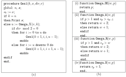
ProcedureGen1in Figure 1 is a general procedure generating exhaustively the list ofst_-restricted growth sequences, wherest_{is a statistic satisfying relations (2) and (3). According to particular} instances of the functionOmega Xcalled by it (and so, of the statisticst_{),Gen1produces specific} st_{-restricted growth sequences, and in particular the listsSEn,An,Rn, andSn. From the length} one sequence 0,Gen1constructs recursively increasing lengthst_{-restricted growth sequences: for} a given prefix s1s2. . . sk it produces all prefixes s1s2. . . ski, with i covering (in increasing or decreasing order) the defining set of s1s2. . . sk; and eventually all length nst-restricted growth sequences. It has the following parameters:

• k, the position in the sequences _{which is updated by the current call;}

• x, belongs to the defining set of s1s2. . . sk−1, and is the value to be assigned to sk;

• dir, the direction (ascending for dir mod 2 = 0 and descending for dir mod 2 = 1) to cover the defining set ofs1s2. . . sk−1;

• v, the value of the statistic of the prefix s1s2. . . sk−1 from which the value of the statistic

of the current prefixs1s2. . . sk is computed. Remark thatv=ωX(s1s2. . . sk−1)−1.

FunctionOmega XcomputesωX(s1s2. . . sk) (see relation (5)), and the main call isGen1(1,0,0,0). In Gen1the amount of computation of each call is proportional with the degree of the call, and there are no degree one calls, and so it satisfies the CAT principle stated at the end of Section 2, and so it is an efficient generating algorithm. The computational tree of Gen1producing the listA4 is given in Figure 2. Each node at level k, 1≤k≤4, represents prefixess1s2. . . sk, and

procedure Gen1(k, x, dir, v) global: n,s_;

sk:=x;

ifk=n then Prints_;

elseu:=Omega X(v, k);

ifdir mod 2 = 0

then fori:= 0to u do

Gen1(k+ 1, i, i, u−1);

enddo

else fori:=udownto 0do

Gen1(k+ 1, i, i+ 1, u−1);

enddo endif

end.

(a)

(i) function Omega SE(w, p)

returnp;

end.

(ii)function Omega A(w, p)

if p >1 andsp > sp₋1 then returnw+ 2;

else returnw+ 1;

endif end.

(iii)function Omega R(w, p)

if p >1 andsp> w then returnw+ 2;

else returnw+ 1;

endif end.

(iv)function Omega S(w, p)

returnsp+ 1;

end.

(b)

Figure 1: (a) AlgorithmGen1, generating the listXn; (b) Particular function Omega Xcalled by Gen1, and returning the value for ωX(s1s2. . . sk), ifXn is one of the sets: (i) SEn, (ii)An, (iii) Rn, and (iv)Sn.

Figure 2: The tree induced by the initial call Gen1(1,0,0,0) for n= 4 and generating the list

4

The Co-Reflected Gray Code order for the sets

SE

_n

_,

A

_n

_,

R

_n

_,

and

S

_n

In this section we will consider, as in the previous one, the sets SEn,An,Rnand Sn, but listed in ≺c order. Our main goal is to prove that the obtained lists are Gray codes as well, and to develop generating algorithms for these lists. Recall thatXn generically denotes one of the sets SEn,An,Rn, or Sn; and letXen denote their corresponding list in≺c order, that are,SEfn,Aen,

e

Rn, or Sen. Clearly, a set of sequences listed in ≺c order is a suffix partitioned list, that is, all sequences with same suffix are contiguous, and such are the lists we consider here.

For a setXnand a sequenceb_{=bk+1bk+2. . . bn, we call} b_{an admissible suffix inXnif there}

exists at least a sequence in Xn having suffixb_{. For example, 124 is an admissible suffix inA6,}

because there are sequences in A6 ending with 124, namely 012124 and 010124. On the other

hand, 224 is not an admissible suffix inA6; indeed, there is no length 6 ascent sequence ending

with 224.

We denote by Xen|bthe sublist of Xen of all sequences having suffixb, and clearly, Xen|bis a contiguous sublist of Xen. The set of all x such that xb is also an admissible suffix in Xn is called the defining set of the suffixb_.

For ≺ order discussed in Section 3, the characterization of prefixes is straightforward: a1a2. . . ak is the prefix of some sequences in Xn, n > k, if and only if a1a2. . . ak is in Xk.

And the defining set of the prefixa1a2. . . ak is {0,1, . . . ,st(a1a2. . . ak) + 1}. In the case of ≺c order, it turns out that similar notions are more complicated: for example, 13 is an admissible suffix inA5, but 13 is not inA2; and the defining set of the suffix 13 is {0,2}, because 013 and

213 are both admissible suffixes in A5, but 113 is not. See Table 4 for the set A5 listed in ≺c order.

4.1 Suffix expansion of sequences in the sets SE_n, A_n, R_{n, and} S_n

For a suffix partitioned list, we need to buildst_{-restricted growth sequences under consideration} from right to left, i.e., by expanding their suffix. For this purpose, we need the notions defined below.

Definition 5. Letb_{=bk+1bk+2. . . bn, 1≤k < n, an admissible suffix in Xn.}

• αX(b) is the set of all elements in the defining set of the suffixb. Formally:

αX(b) ={x|xbis an admissible suffix in Xn},

and for the empty suffixǫ,αX(ǫ) ={0,1, . . . , n−1}.

• µX(b_{) is the minimum required value of the statistic defining the setXn, and provided by}

a length (k+ 1) prefix of a sequence inXn having suffixb_{. Formally:}

µX(b_{) = min{}st_{(s1s2. . . skbk+1)|s1s2. . . sk}b_∈Xn}.

Notice that µX(xb)∈ {µX(b)−1, µX(b), x} forx∈αX(b).

Proof. If sk < k−1, then in each case for st, st(s1s2. . . sk) < k−1, which is in contradiction withsk+1=k, and so sk=k−1. Similarly, sk−1 =k−2, . . . , s2= 1, and s1 = 0.

Under the conditions in the previous remark, sk+1=kimposes that all values at the left of k+ 1 in s _{are uniquely determined. As we will see later, in the induced tree of the generating}

algorithm, all descendants of a node withsk+1 =k have degree one, and we will eliminate the

obtained degree-one path in order not to alter the algorithm efficiency.

It is routine to check the following propositions. (Actually, Proposition 3 is a consequence of Remark 1.)

Proposition 3. LetXnbe one of the setsSEn,An,Rn, orSn. Ifb_{=bk+1bk+2. . . bn,1≤k < n,}

is an admissible suffix in Xn, then bk+1 ≤µX(b).

Proposition 4. Let Yn be one of the setsAn, Rn, or Sn. If b_{=bk+1bk+2. . . bn, 1≤k < n, is}

an admissible suffix inYn, then

1 if b_{=bn, that is, a length one admissible suffix, thenµY(}b_{) =bn;}

2 µY(b_{) =k if and only if bk+1=k;}

3 if xb_{is also an admissible suffix in Yn (i.e., x∈αY(}b_{)) and x≥bk+1, then}

µY(xb_{) = max{x, µY(}b_)}.

The following propositions give the values for αX(b_{) and µX(x}b_{), if Xn is one of the sets}

SEn, An, Rn, or Sn. We do not provide the proofs for Propositions 5, 6, 11, and 12, because they are obviously based on the definition of the corresponding sequences.

Proposition 5. Let b_=ǫor b_{=bk+1bk+2. . . bn be an admissible suffix in SEn. Then}

αSE(b) =

{0,1, , . . . , n−1} if b_=ǫ,

{0,1, . . . , k−1} otherwise.

Proposition 6. Let b_{=bk+1bk+2. . . bn be an admissible suffix in SEn and x∈αSE(}b_{). Then}

µSE(xb_{) =µSE(}b_)−1.

Obviously, for a length one suffixb_{=bn, it follows thatµSE(}b_{) =n−1.}

Example 2. If b_{=ǫ, and n= 10, then αSE(}b_{) ={0,1, . . . ,9};}

and for b_{=b10, b10∈ {0,1, . . . ,9}, it follows that µSE(x}b_{) = 9−1 = 8, for all x∈αSE(}b_).

Proposition 7. Let b_=ǫor b_{=bk+1bk+2. . . bn be an admissible suffix in An. Then}

αA(b_{) =}

      

{0,1, . . . , n−1} if b_=ǫ,

{k−1} if µA(b_{) =k, or µA(}b_{) =k−1 and bk+1= 0,}

{0,1, . . . , bk+1−1} ∪ {k−1} if µA(b) =k−1 and 0< bk+1< k,

Proof. If b_{=ǫ, the result is obvious.}

Forb_{6=ǫ, let x∈αA(}b_).

IfµA(b_{) =k, by Proposition 4 point 2,bk+1=kand by Remark 3 we have x=k−1.}

IfµA(b_{) =k−1 and bk+1= 0, then} asc_{(xbk+1) = 0, and soµA(x}b_{) =µA(}b_{) =k−1, and again}

by Proposition 4 point 2 we have x=k−1.

IfµA(b_{) =k−1 and 0< bk+1 < k, then there are two possibilities forµA(x}b_):

• µA(xb_{) =µA(}b_{) =k−1, if}asc_{(xbk+1) = 0, and as above x=k−1;}

• µA(xb) =µA(b)−1 =k−2, ifasc(xbk+1) = 1. In this case x∈ {0,1, . . . , bk+1−1}.

IfµA(b_{)< k−1 (and consequently 0≤bk+1 < k), then there are two possibilities for µA(x}b_):

• µA(xb_{) =µA(}b_{), if} asc_{(xbk+1) = 0, and we have x∈ {bk+1, bk+1+ 1, . . . , k−1};}

• µA(xb_{) =µA(}b_{)−1, if}asc_{(xbk+1) = 1, and we have x∈ {0,1, . . . , bk+1−1}.}

Proposition 8. Let b_{=bk+1bk+2. . . bn be an admissible suffix in An and x∈αA(}b_{). Then}

µA(xb_{) =}

  

x if x≥µA(b_),

µA(b_{) if bk+1 ≤x < µA(}b_),

µA(b_{)−1 if x < bk+1.}

Proof. If x ≥µA(b), by Proposition 3 it follows that x ≥ bk+1, and by Proposition 4 point 3,

thatµA(xb_{) = max{x, µA(}b_)}=x.

Ifbk+1≤x < µA(b), then, again by Proposition 4 point 3, it follows thatµA(xb) = max{x, µA(b)}= µA(b).

Ifx < bk+1, then asc(xbk+1) = 1, soµA(xb) =µA(b)−1.

Example 3. Let k= 5, n= 9, and b_{=b6b7b8b9 = 2050 be an admissible suffix inA9. Clearly,}

µA(b_{), the minimum number of ascents in a prefix s1s2. . . s5b6 such that s1s2. . . s5}b_{∈A9, is 4.}

In this case, denoting s5 by x, we have

• the set αA(b_{) of all possible values for x is{0,1, , . . . , bk+1−1} ∪ {k−1}={0,1} ∪ {4}.}

• µA(xb_{) =µA(}b_{)−1 = 4−1 = 3, if x∈ {0,1}; orµA(x}b_{) =µA(}b_{) = 4, if x= 4.}

Proposition 9. Let b_=ǫor b_{=bk+1bk+2. . . bn be an admissible suffix in Rn. Then}

αR(b_{) =}

  

{0,1, . . . , n−1} if b_=ǫ,

{k−1} if µR(b_{) =k, or µR(}b_{) =k−1 and bk+1< k−1,}

{0,1, . . . , k−1} if µR(b) =k−1 and bk+1 =k−1, or µR(b)< k−1. Proof. If b_{=ǫ, the result is obvious.}

Forb_{6=ǫ, let x∈αR(}b_).

IfµR(b_{) =k, by Proposition 4 point 2,bk+1 =kand by Remark 3 we have x=k−1.}

If µR(b_{) =k−1 and bk+1 < k−1, then the maximal value of the statistic} m_{(defining the set} Rn) of a lengthk+ 1 prefix ending withbk+1 < k−1 is k−1, and it is reached whenx=k−1.

• µR(xb) =µR(b) =k−1, and as above, this impliesx=k−1;

• µR(xb_{) =µR(}b_{)−1 =k−2, which implies x∈ {0,1, . . . , k−2}.}

Finally, if µR(b_{)< k−1, then x can be any value in{0,1, . . . , k−1}.}

Proposition 10. Let b_{=bk+1bk+2. . . bn be an admissible suffix inRn and x∈αR(}b_{). Then}

µR(xb_{) =}

  

x if x≥µR(b_),

µR(b_{) if bk+1 ≤x < µR(}b_{) or x < bk+1 < µR(}b_),

µR(b_{)−1 if x < bk+1=µR(}b_).

Proof. The case x≥µR(b_{) is analogous with the similar case in Proposition 8.}

The next case is equivalent withx < µR(b_{) and bk+1< µR(}b_{), and sinceRn corresponds to the}

statistic m_{, the result holds.}

Finally, if x < bk+1 =µR(b), then µR(b) =µR(xb) + 1, and so µR(xb) =µR(b)−1.

Example 4. Let k= 4, n= 7, and b_{=b5b6b7 = 241 be an admissible suffix in R7. It follows}

that bk+1= 2, µR(b) = 3 and

• αR(b) ={k−1}={3};

• µR(xb_{) =x= 3.}

Proposition 11. Let b_=ǫor b_{=bk+1bk+2. . . bn be an admissible suffix inSn. Then}

αS(b) =

  

{0,1, . . . , n−1} if b_=ǫ,

{k−1} if bk+1 =k,

{C, C+ 1, . . . , k−1} if 0≤bk+1 ≤k−1,

where C = max{0, bk+1−1}.

Since µS(b_{) =bk+1, the next result follows:}

Proposition 12. Let b_{=bk+1bk+2. . . bn be an admissible suffix inSn and x∈αS(}b_{). Then}

µS(xb_{) =x.}

Example 5. Let k= 6, n= 9, and b_{=b7b8b9 = 457 be an admissible suffix inS9. So we have}

µS(b) = 4, C= max{0, bk+1−1}= max{0,3}= 3, and

• αS(b_{) ={C, C+ 1, . . . , k−1}={3,4,5};}

• µS(xb_{) =x, where x∈ {3,4,5}.}

4.2 The bound of Hamming distance between successive sequences in the lists SEfn, Aen, Ren, and Sen

4.2.1 The list SEfn

Theorem 2. The list SEfn is 1-Gray code.

Proof. The result follows from the fact that the restriction of the 1-Gray code list Gn(n) to any product space remains a 1-Gray code (see [13]), in particular to the set

Vn=ϑ1×ϑ2×. . .×ϑn,

where

• ϑi={0,1, ..., n−i}, ifnis odd and iis even, or

• ϑi={i−1, i, ..., n−1}, ifnis even, orn andi are both odd.

Then by applying to each sequence s _{in the list Vn the two transforms mentioned before}

Definition 2, namely:

• complementing each digit ins_{ifnis even, or only digits in odd positions ifnis odd, then}

• reversing the obtained sequence,

the desired 1-Gray code for the setSEn in≺c order is obtained.

4.2.2 The lists Aen and Ren

The next proposition describes the pattern of s_{= last(Y}e_{n |}b_{) and} s_{= first(Y}e_{n |}b_{), where Y}e_n

is one of the lists Aen or Ren.

Proposition 13. Let Yn be one of the sets An or Rn, and b=bk+1bk+2. . . bn be an admissible suffix inYn. If s_{= last(Y}e_{n |}b_{) or} s_{= first(Y}e_{n |}b_{), then} s_{has one of the following patterns:}

• s_{= 012. . .(k−2)(k−1)}b_{, or}

• s_{= 012. . .(k−2)0}b_.

Proof. Lets_{=s1s2. . . skbk+1bk+2. . . bn. Since}s_{= last(Y}e_{n |}b_{) ors= first(Y}e_{n |}b_{), according to}

αY(b) given in Propositions 7 and 9, it follows thatsk∈ {0, k−1}. In other words,sk is either the smallest or the largest value in αY(b_).

Ifsk=k−1, then by Remark 3 we haves= 012. . .(k−2)(k−1)b. Ifsk= 0, then considering the definition of ≺c order we have either

• s_{= first(Y}e_{n |}b_{) and} Pn

i=k+1bi+ (n−k) is odd, or

• s_{= last(Y}e_{n |}b_{) and} Pn

i=k+1bi+ (n−k) is even.

For the first case, again by the definition of ≺c order, it follows that sk−1 must be the largest

value in αY(0b_{), and so sk}

−1 = k−2, and by Remark 3, s = 012. . .(k−2)0b. Similarly, the

same result is obtained for the second case.

A direct consequence of the previous proposition is the next theorem.

Proof. Let s_,t_{∈Yn, with}t_=succgY(s_{). If k+ 1 is the rightmost position where}s _and t_differ,

then there are admissible suffixes b _{= bk+1bk+2. . . bn and} b′ _{= b}′

k+1bk+2. . . bn in Yn such that

s_{= last(Y}e_n|b_{) and} t_{= first(Y}e_n|b′_).

By Proposition 13,s_{has pattern}

012. . .(k−2)(k−1)b_{, or}

012. . .(k−2)0b_;

and t_{has pattern}

012. . .(k−2)(k−1)b′_{, or}

012. . .(k−2)0b′_.

And in any case, s_and t_{differ in position k+ 1 and possibly in positionk.}

4.2.3 The list Sen

The next proposition gives the pattern of last(Sen |b) and first(Sen |b) for an admissible suffixb inSn.

Proposition 14. Let b_{=bk+1bk+2. . . bn be an admissible suffix in Sn. If} s_{= last(S}e_{n |}b_{), then}

the pattern of s_{is given by:}

• if bk+1=kor Pn_i=k+1bi+ (n−k) is odd, then

s_{= 012. . .(k−2)(k−1)}b_;

• if bk+1< k and Pn_i=k+1bi+ (n−k) is even, and eitherbk+1 = 0 or bk+1 is odd, then

s_{= 012. . .(k−2)(max{0, bk+1−1})}b_;

• if bk+1< k and Pn_i=k+1bi+ (n−k) is even, and bk+1>0 is even, then

s_{= 012. . .(k−3)(bk+1−2)(bk+1−1)}b_.

Similar results hold for s _{= first(S}e_{n |}b_{) by replacing ‘odd’ by ‘even’, and vice versa, for the}

parity of Pn_i=k+1bi+ (n−k).

Proof. Let s_{=s1s2. . . skbk+1. . . bn= last(S}e_{n |}b_).

If bk+1 =kor Pn_i=k+1bi+ (n−k) is odd, then sk is the largest value in αS(b), sosk=k−1, and by Remark 3,si =i−1 for 1≤i≤k. So the first case holds.

If Pn_i=k+1bi + (n−k) is even and bk+1 < k, then sk is the smallest value in αS(b), namely max{0, bk+1−1}, which is even if bk+1 = 0 or bk+1 is odd. Thus, by the definition of ≺c order, sk₋1 is the largest value in αS(skb), which isk−2, and by Remark 3, the second case holds.

For the last case, as above, sk= max{0, bk+1−1}, and consideringbk+1>0 and even, it follows

thatsk=bk+1−1 is odd. Thussk−1 is the minimal value inαS(skb), that is bk+1−2, which in

turns is even, and the last case holds.

The proof for the cases_{= first(S}e_{n |}b_{) is similar.}

Proof. Lett_=succgS(s_{), andk+ 1 be the rightmost position where}s_andt_{differ. Let us denote}

by b_{the length (n−k) suffix of} s_and b′ _{that of}t_{; so,} s_{= last(}b_{| Sn) and}t_{= first(}b′_{| S}

n). It follows by Proposition 14, that si = ti = i−1 for all i ≤ k−2, and so the other differences possibly occur in positionk and in positionk−1.

Considering all valid combinations for s _and t _{as given in Proposition 14, the proof of the}

adjacency is routine, and based on the following: sk6=tk if and only if sk₋1 6=tk₋1. It follows

thats _andt _{differ in one position, or three positions which are adjacent.}

In addition, the lists Aen,Ren, and Sen, are circular Gray codes. This is a consequence of the following remarks based on Propositions 13 and 14:

• first(Yen) = 012. . .(n−2)(n−1);

• last(Yen) = 012. . .(n−2)0;

whereYenis one of the lists Aen,Ren, orSen.

4.3 Generating algorithm for SEfn, Aen, Ren, and Sen

Here we explain algorithm Gen2 in Figure 3 which generates suffix partitioned Gray codes for restricted growth sequences; according to particular instances of the functions called by it,

Gen2 produces the list SEfn, Aen, Ren, or Sen. Actually, for convenience, Gen2 produces length (n+ 1) sequences s _{= s1s2. . . sn+1 with sn+1 = 0, and so, neglecting the last value in each}

sequence s _{the desired list is obtained. Notice that with this dummy value for sn+1 we have}

µX(sksk+1. . . sn) =µX(sksk+1. . . sn0), for k≤n, and similarly for αX.

In Gen2, the sequence s_{is a global variable, and initialized by 01. . .(n−1)0, which is the}

first length n sequence in ≺c order, followed by a 0; and the main call is Gen2(n+ 1,0,0,0). ProcedureGen2 has the following parameters (the first three of them are similar with those of procedureGen1):

• k, the position in the sequences _{which is updated by the current call;}

• x, the value to be assigned to sk;

• dir, gives the direction in which sk₋1 covers αX(sksk+1. . . sn0), the defining set of the

current suffix;

• v, the value ofµX(sk+1. . . sn0).

The functions called by Gen2are given in Figures 4 and 5. They are principally based on the evaluation ofαX and µX for the current suffix of s_{, and are:}

• Mu X(k, x, v) returns the value of µX(sksk+1. . . sn0), with x=sk.

• IsDegreeOneX(k) stops the recursive calls whenαX(sksk+1. . . sn0) has only one element,

namelyk−2. In this case, by Remark 3 the sequence is uniquely determined by the current suffix, and this preventsGen2to produce degree one calls. In addition,IsDegreeOne X(k) sets appropriatellyd−1 values at the left ofsk, wheredis the upper bound of the Hamming distance in the list (changes at the left of s1 are considered with no effect). This can be

• LowestX(k) is called when IsDegreeOneX returns false, and gives the lowest value in αX(sksk+1. . . sn0).

• SecLargest X(k, u), is called when IsDegreeOne X returns false, and gives the second largest value inαX(sksk+1. . . sn0) (the largest value being always k−2).

By this construction, algorithm Gen2has no degree one calls and it satisfies the CAT principle.

Figure 6 shows the tree induced by the algorithm when generatesAe4.

procedure Gen2(k, x, dir, v)

global n,s_;

sk:=x;

u:=Mu X(k, x, v); if IsDegreeOne X(k, u) then Print s_;

else c:=Lowest X(k);

d:=SecLargestX(k, u); if dir mod 2 = 1

then for i:=c to d do Gen2(k−1, i, i, u); enddo

endif

Gen2(k−1, k−2,(k−1−dir) mod 2, u); if dir mod 2 = 0

then for i:=d downto c do Gen2(k−1, i, i+ 1, u); enddo

endif endif end.

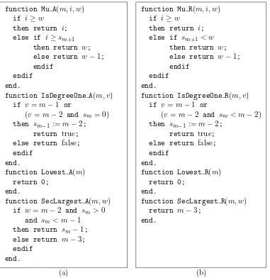
function Mu A(m, i, w)

function Mu S(m, i, w)

return i; end.

function IsDegreeOne S(m, v)

if sm=m−1

then sm₋1 :=m−2; sm₋2 :=m−3; return true; else return false; endif

end.

function Lowest S(m)

if sm>1 and sm ≤m−2

then return sm−1; else return 0; endif

end.

function SecLargest S(m, w) return m−3;

end.

function Mu SE(m, i, w)

if m=n

then return n−1; else return w−1; end.

function IsDegreeOne SE(m, v)

if m= 2

then return true; else return false; end.

function Lowest SE(m)

return 0; end.

function SecLargest SE(m, w)

return m−3; end.

(a) (b)

Figure 5: Particular functions called byGen2, generating the lists: (a)Sen, and (b)SEfn.

5

Final remarks

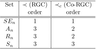
We conclude this paper by comparing for each of the sets SEn, An, Rn and Sn the prefix partitioned Gray codes induced by ≺order and the suffix partitioned one induced by≺c order. This can be done by comparing the Hamming distance between all pairs of successive sequences either in the worst case or in average.

Table 1 summarizes Theorems 1, 3, and 4, and Proposition 2, and gives the upper bound of the Hamming distance (that is, the worst case Hamming distance) for the two order relations. It shows that for the sets SEn and Sn these relations have same performances, and for the sets An and Rn,≺c order induces more restrictive Gray codes.

Set ≺(RGC) ≺c (Co-RGC) order order

SEn 1 1

An 3 2

Rn 3 2

Sn 3 3

Table 1: The bound of the Hamming distance between two successive sequences in ≺ and ≺c orders.

For a list L of sequences, theaverage Hamming distance is defined as

P

d(s_,t₎

N −1 ,

where the summation is taken over all s_{in L, except its last element,} t_{is the successor of} s _in

L,dis the Hamming distance, and N the number of sequences in L.

Surprisingly, despite ≺c order has same or better performances in terms of worst case Hamming distance, if we consider the average Hamming distance, numerical evidences show that ≺ order is ‘more optimal’ than ≺c order on An, Rn (n ≥ 5), and Sn (n ≥ 6). And this phenomenon strengthens for largen; see Table 2.

n

≺(RGC) order ≺c (Co-RGC) order

SEn An Rn Sn SEfn Aen Ren Sen

4 1 1.21 1.21 1.31 1 1.14 1.14 1.15 5 1 1.13 1.12 1.29 1 1.19 1.18 1.24 6 1 1.09 1.07 1.27 1 1.23 1.20 1.31 7 1 1.06 1.06 1.26 1 1.25 1.22 1.35 8 1 1.04 1.04 1.25 1 1.26 1.23 1.37 9 1 1.03 1.03 1.24 1 1.28 1.24 1.39 10 1 1.02 1.03 1.23 1 1.28 1.24 1.41

Table 2: The average Hamming distance for≺order and ≺c order.

Algorithmically, ≺c order has the advantage that its corresponding generating algorithm, Gen2, is more appropriate to be parallelized than its ≺ order counterpart, Gen1. Indeed, the

main call ofGen1), and so we can have more parallelized computations; and this is more suitable for large n. See Figure 2 and 6 for examples of computational trees.

Finally, it will be of interest to explore order relation based Gray codes for restricted growth sequences defined by statistics other than those considered in this paper. In this vein we suggest the following conjecture, checked by computer for n ≤ 10, and concerning descent sequences (defined similarly with ascent sequences in Section 2).

References

[1] Gray, F. (1953) Pulse code communication, U.S. Patent 2632058 .

[2] Er, M.C. (1984) On generating the N-ary reflected Gray code, IEEE Transaction on Computers,33(8), 739–741.

[3] Bernini, A., Grazzini, E., Pergola, E. and Pinzani, R. (2007) A general exhaustive generation algorithm for Gray structures,Acta Informatica, 44(5), 361-376.

[4] Vajnovszki, V. (2010) Generating involutions, derangements, and relatives by ECO, DMTCS, 12 (1), 109-122.

[5] Ruskey, F. and Williams, A. (2009) The coolest way to generate combinations, Discrete Mathematics,309, 5305-5320.

[6] Ruskey, F., Sawada, J. and Williams, A. (2012) Binary bubble languages, Journal of Combinatorial Theory, Ser. A 119(1), 155-169.

[7] Klingsberg, P. (1981) A Gray code for compositions,Journal of Algorithms, 3 (1), 4144.

[8] Walsh, T. (2000) Loop-free sequencing of bounded integer compositions, Journal of Combinatorial Mathematics and Combinatorial Computing,33, 323-345.

[9] Baril, J.-L. and Vajnovszki, V. (2005) Minimal change list for Lucas strings and some graph theoretic consequences,Theoretical Computer Science, 346, 189-199.

[10] Vajnovszki, V. (2001) A loopless generation of bitstrings without p consecutive ones, Discrete Mathematics and Theoretical Computer Science- Springer, 227-240.

[11] Vajnovszki, V. (2007) Gray code order for Lyndon words, Discrete Mathematics and Theoretical Computer Science,9 (2), 145-152.

[12] Vajnovszki, V. (2008) More restrictive Gray codes for necklaces and Lyndon words, Information Processing Letters,106, 96-99.

[13] Vajnovszki, V. and Vernay, R. (2011) Restricted compositions and permutations: from old to new Gray codes,Information Processin Letters,111, 650-655.

[14] Mansour, T. and Vajnovszki, V. (2013) Efficient generation of restricted growth words, Information Processing Letters,113, 613-616.

[15] van Baronaigien, D.R. and Ruskey, F. (1993) Efficient generation of subsets with a given sum,JCMCC,14, 87-96.