Linear programming system identification pdf

Continuous Optimization

Linear programming system identification

Marvin D. Troutt

a,*

, Suresh K. Tadisina

b,1

, Changsoo Sohn

c,2

,

Alan A. Brandyberry

d,3

a

Department of Management and Information Systems, Kent State University, Kent, OH 44242-0001, USA b

Department of Management, Southern Illinois University, Carbondale, IL 62901-4627, USA c

Department of Business Administration, School of Business Administration, The Catholic University of Korea, San 43-1, Yokkok 2-Dong, Wonmi-Gu, Puchon City, Gyuonggi-Do 420-743, South Korea

d

Department of Management and Information Systems, Kent State University, Kent, OH 44242-0001, USA

Received 22 February 2002; accepted 30 July 2003 Available online 13 December 2003

Abstract

We define a version of the Inverse Linear Programming problem that we call Linear Programming System Iden-tification. This version of the problem seeks to identify both the objective function coefficient vector and the constraint matrix of a linear programming problem that best fits a set of observed vector pairs. One vector is that of actual decisions that we call outputs. These are regarded as approximations of optimal decision vectors. The other vector consists of the inputs or resources actually used to produce the corresponding outputs. We propose an algorithm for approximating the maximum likelihood solution. The major limitation of the method is the computation of exact volumes of convex polytopes. A numerical illustration is given for simulated data.

Ó _{2003 Elsevier B.V. All rights reserved.}

Keywords:Inverse optimization; Linear programming; Parameter estimation; Constraint matrix estimation; Maximum likelihood

1. Introduction

Linear programming (LP) is perhaps the most widely applicable technique in Operational Re-search. However, obtaining the parameters,

namely, the objective function coefficients and technological coefficient matrix, is typically the most difficult step of a modeling project based on LP. The method proposed here can estimate the LP objective coefficient vector and the technolog-ical coefficient matrix from time series or cross-sectional data on actual decisions and resources used. We call the actual decisions outputs and similarly, we call the resources inputs. Thus, given data on output vectors and input vectors we wish to infer the best fitting LP model.

This problem lies in the class known as inverse optimizationand can be referred to as an instance ofInverse LP. Tarantola (1987) has given a general

*_{Corresponding author. Tel.: 672-1145; fax:} +1-330-672-2953.

E-mail addresses: mtroutt@kent.edu (M.D. Troutt), sur-esht@siu.edu (S.K. Tadisina), csohn@catholic.ac.kr (C. Sohn), abrandyb@kent.edu (A.A. Brandyberry).

1_{Tel.: +618-453-3307.} 2_{Tel.: +8232-340-3287.}

3_{Tel.: +330-672-1146; fax: +330-672-2953.}

0377-2217/$ - see front matter Ó 2003 Elsevier B.V. All rights reserved. doi:10.1016/j.ejor.2003.07.019

account of inverse problem solving and discusses several applications, particularly in the physical sciences. Although LP is used in that work for algorithmic steps, the Inverse LP problem itself was not addressed. On the other hand, Zhang and Liu (1996), and Ahuja and Orlin (2001), respec-tively, have treated versions of the Inverse LP problem. Zhang and Liu (1996) considered inverse assignment and minimum cost flow problems. Ahuja and Orlin (2001) studied a more general LP problem and a version of the problem as follows. Given a feasible solution x0, find the minimum

perturbation of the objective function coefficients so thatx0becomes an optimal solution. Solutions

to this problem were obtained for both theL1- and

L1-norms. In this paper, we consider a version of the inverse LP problem that seeks estimates of

both the objective function vector and the con-straint matrix coefficients from a sample of ob-served resource vectors and decision vectors. We call this versionLP system identification.It may be stated formally following some notational con-ventions.

Notational conventions: Vectors and matrices are written in boldface fonts. Vectors are column vectors. The transpose of vectoryis denoted byy0_. We denote bymðÞthe volume (Lebesgue measure) of a set (Æ). We abbreviate the terms, probability density function(s), as pdf(s). Similarly, we abbreviate the term, cumulative distribution function, by cdf.

We may now state the problem formally. Sup-pose that for each observation index t¼1;. . .;T

there are given data on output or decision vectors

yt_{, with components y}t

r, r¼1;. . .;R and input

vectors, xt_{, with componentsx}t

i,i¼1;. . .;I.

Sup-pose further that (1) there exists a nonnegative technological coefficient matrix A¼ fairg, such that Ayt6xt _{for all t; and (2) there exists a}

non-negative objective coefficient vector p with com-ponents pr, such that the observed yt-vectors

approximate, in a sense to be defined below, optimal solutions of the linear programming problemsPt given by

Pt: max p0y;

s:t: Ayt

6xt _{for all}

t and

yP0 componentwise:

ð1:1Þ

Letyt _{denote any optimal solution to problemPt.}

Then the ratio

vt¼p0yt₌

p0yt _ð1:2Þ

is a measure of the degree to which the actual performance for observation t achieves its maxi-mum value. Such ratios are instances ofdecisional efficiencymeasures as proposed in Troutt (1995). In that paper, a method of parameter estimation called the maximum decisional efficiency (MDE) principle was proposed. This paper applies the MDE principle to solve the sub-problems of esti-matingp givenAas Avaries over a set of admis-sible choices. Following estimation of p given A, the imputed value of the ratios in (1.2) may be obtained. A pdf can then be fitted to these ratios, and a joint pdf can be constructed for the set of feasible output vectors for each linear program-ming problem Pt. From these pdfs, a likelihood score can be obtained for the observed sample. Thus, we develop a maximum likelihood approach for the joint estimation ofpandA.

The rest of the paper is organized as follows. Section 2 discusses the Maximum Decisional Effi-ciency principle and a maximin estimation model derived from it. In Section 3, a method for repre-senting the set of admissible or candidate A -matrices is proposed. Section 4 develops a joint likelihood function for the sample of output vec-tors. In terms of the above notations, this likeli-hood is a function of the data and parameters denoted by Lðy1_;

. . .;yt_;x1_;

. . .;xt_{jp;AÞ. Section 5}

summarizes the estimation method in pseudo-code form and provides a numerical illustration on simulated data. Section 6 provides a discussion of limitations and potential extensions, and Section 7 provides conclusions.

2. Overviews of the strategy and maximum deci-sional efficiency estimation

general MDE method, the MMA model is derived. Then the space of admissible A-matrices is con-structed in Section 3. A likelihood score is asso-ciated to eachAandp pair in Section 4 and the space of admissibleA-matrices is searched for the pair (A, p ðAÞ) with the largest likelihood. Thus, we propose a maximum likelihood procedure for the joint estimation ofp andA.

For the derivation of the MMA model below, it is useful to briefly review the MDE estimation principle in general form as discussed in Troutt (1995). Let fðx;pÞ be an objective function depending on an unknown, or perhaps imprecisely known, parameter vector,p. LetX Rn _be

com-pact, and let P Rm _{be compact. Assume}

fðx;pÞP0 for all x2X and p2P. Finally, let

x ðpÞbe any solution of max fðx;pÞ. Then define the decisional efficiency,vt_{, of observation, x}t_{, by}

vt_¼vt_{ðpÞ ¼fðx}t_{;pÞ=fðx ðpÞ;pÞ: ð2:1Þ}

Clearly, 06vt_{ðpÞ61for all p2P. Thus, v}t_ðpÞ

measures the degree of optimality of the observed decision, xt_{, as a function of the unknown}

parameter vector,p. Since it is also the ratio of an actual return or benefit to maximum potential one, it can be regarded as an efficiency measure, hence, the termdecisional efficiency.

In the case of one observation, the MDE prin-ciple chooses the estimate of the true value ofpas thatp0 _{for which}

vðp0Þ ¼maxvðpÞ: ð2:2Þ

To extend the notion to multiple observations, let

vðpÞbe the vector with componentsvt_{ðpÞ. Letrbe}

an aggregator function such as the sum, mean, geometric mean, minimum (Leontif), etc. Then the MDE principle estimates the true value ofpbyp0

wherep0_{is the parameter vector that maximizes the}

aggregate decisional efficiencyrfvðpÞg. For exam-ple, if we choose summation as the aggregator, then the MDE estimatep0_maximizesPT

t¼1vtðpÞ.

We next model the main sub-problem for p ¼pðAÞ using the MDE approach. We select the minimum aggregator, which results in a maximin formulation. The MDE sub-problem for pgivenAis given by

max min

t p

0_yt_=p0_yt _{: ð2:3Þ}

By LP duality, we also have

p0yt _¼nt 0_xt_{; ð2:4Þ}

where the nt are the optimal dual variables for problem Pt. Therefore, the decisional efficiency vt

for observation tcan be expressed as

vt¼p0yt_=nt 0_xt_{; ð2:5Þ}

wherent 0_xt_{is the optimal solution to the dual}

prob-lemDtassociated withPt, and whereDtis given by

Dt: min nt0xt_{; ð2:6Þ}

s:t: A0nt¼p; ð2:7Þ

ntP0 componentwise: ð2:8Þ We have chosen the constraints (2.7), as opposed to A0ntPp, for the following reason. We assume that all data vectorsyt _{have strictly positive}

com-ponents. In turn, we assume that the unobserved

yt _{-vectors also have strictly positive components.}

Since these yt _{-vectors may be considered as the}

dual variables for the constraints (2.7), the slack variables of the constraints A0ntPp must be zero by complementary slackness.

Next, we note that a normalization is necessary. Namely, if p is replaced bykp in problems,Pt or

Dt, where k>0, then the corresponding dual variables are also multiplied bykwithout changing the value of the efficiency ratios vt_{. For this}

pur-pose, we choose the normalization constraint

nt0 0_xt0 _{¼1; ð2:9Þ}

wheret0is a particular index choice.

Finally, it is necessary to insure that the effi-ciency ratios do not exceed unity. This can be accomplished by including the constraints

p0yt6nt 0_xt _{for allt: ð2:10Þ}

Collecting these considerations, the estimation model for thepgivenAsub-problem is then given by model MMA.

MMA: max min

t p

0_yt₌

nt0xt; ð2:11Þ

s:t: A0nt¼p componentwise for allt; ð2:12Þ p0yt6nt0xt for allt; ð2:13Þ

nt00_xt0_{¼1; ð2:14Þ}

It is important to note that the maximization of the minimum ratio in (2.9) requires that nt0xt _be

simultaneously minimized, which together with constraints (2.10) and (2.13), make the resultingnt

optimal for the problemsDt, corresponding to the vectorp. In particular, whenp is the optimal p -solution for problem MMA, then the associated optimal nt can be seen to be the corresponding optimal dual variables nt .

Model MMA is a generalized fractional pro-gramming problem for which several algorithms have been proposed. See, for example, Crouzeix et al. (1985), Crouzeix and Ferland (1991), Parda-los and Phillips (1991), Barros et al. (1996a,b) and Gugat (1996). However, it is also amenable to solution by general-purpose nonlinear program-ming algorithms such as the GRG2 nonlinear solver in Microsoft ExcelTM_{. For the numerical}

illustration below, a further simplification is shown by which the MMA model can be reduced to a linear programming problem.

3. Generation of the admissible candidate constraint matrices

It is useful to limit the class from which esti-mates of theA-matrix can be chosen.

Definition 1. We call matrix A a technically effi-cient constraint matrix if (i) Ayt6xt

component-wise for all t, (ii) the elements of A are nonnegative, and (iii) Ayt¼xt _{for at least one}

index-t, for each index-i.

The aim of Definition 1is to limit the search to those nonnegative matrices that are ‘‘tight fitting’’ as discussed further below. This class of matrices can be represented with the help of:

Definition 2. We call K¼ fkirg a constraint gen-erator matrix if kirP0 for all i and r, and

P

rkir¼1for alli. For each row-i, define scalars j_i calledrow scale factors, by

j_i ¼min vector. Finally, we define the corresponding admissibleA-matrix by

A¼ fairg ¼ fj_ikirg: ð3:2Þ

Thus, vector ki determines the orientation of the ith constraint hyper-plane, andj_i is a scale factor so that the constraint P

rairy

the tightest fitting half-plane, which encloses all data vectors. Thus by tightest fitting, we mean that the constraint forms the smallest half-space that includes all of the data.

Representation of the K-matrix can be further simplified as follows. Define variables, uir, for

i¼1;. . .;I andr¼1;. . .;R1, as follows. First, By discretizing the interval for each uir into N -steps, this search space can be refined to any de-sired degree. For example, with N ¼100 and a step size ofN1_{¼0:01, values of uir could be}

se-lected from f0:01;0:02;. . .;1:00g. Section 5 gives this process is in detail.

4. Construction of the likelihood function

Let A be a specified candidate matrix. By solution of model MMA, an estimate,p ¼p ðAÞ, can be determined. Also the efficiency ratios

vt_¼vt_{ðAÞ ¼p} 0_yt_=nt

xt_¼p 0_yt_=zt _ð4:1Þ

can then be computed. Thevt_{are distributed over}

the interval½0;1, and a specific pdf model can be fitted to thevt

vectors y, for each problem Pt, as will be seen below. The following additional definitions are needed. Let Ft_{¼ fy:Ay6x}t_{;yrP0 for allrg be}

the set of feasible decision vectorsy, for the prob-lemPt, and letzt _{be the optimal objective function}

value for Pt. Next, let St_ðv;xt_{Þ ¼ fy2F}t_:p0_y¼

vzt _{g. These sets contain those feasible vectors that}

have efficiency scorev. We note that these sets vary witht. This is because, while the constraint matrix

A is the same for each problem Pt, the differing resource data vectorsxt_{create different constraints}

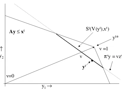
(half-spaces) for eacht. Fig. 1depicts problemPt

and these relationships for the case ofy2R2_.

Next, defineWt_{ðvÞ ¼}S

v0_PvStðv;xtÞas the set of

vectors that are feasible for problemPt, and which also have efficiency scores of v or greater. Also, define the functionsVt_{ðyÞ ¼p}0_y=zt _{. These are}

de-fined on the set of feasible vectors for problemPt

and give the efficiency values of the feasible y -vectors. For example,Vt_ðyt_{Þ ¼v}t_.

We are now able to propose pdf models ft_ðyÞ

for the feasible sets of problems Pt. These pdfs represent the composition of a two-step process. First, a value v, 06v61, is selected according to the pdfgðvÞ. Then givenv, a vectoryis selected on the set St_ðv;xt_{Þ according to the uniform pdf on}

that set. Let Dv be a small positive number and consider the approximation of Probðv6VðyÞ6

vþDvÞin two ways. First, this probability is given by

Z vþDv

v

gðuÞduffigðvÞDv: ð4:2Þ

By the uniform pdf assumption, fðyÞ is constant on St_ðv;xt_{Þfor eachvand has value uðvÞ, say, on}

these sets. It follows that

Probðv6VðyÞ6vþDvÞ

¼

Z

fy:v6VðyÞ6vþDvg

fðyÞY

R

r¼1

dyr

ffiuðvÞ½mðWðv;xÞÞ mðWðvþDv;xÞÞ: ð4:3Þ The volume measure in brackets can be further approximated. For small Dv, it is given by the product of the surface measuremðSt_ðv;xt_{ÞÞand the}

distance element kDv corresponding to Dv and orthogonal toSt_ðv;xt_{Þ. This distance is the length}

of the projection of the vector ðDvÞy in the direction of vector p, which is

ðDvÞz=kpk: ð4:4Þ

It follows that

mðWðv;xÞ mðWðvþDv;xÞ ffimðSt_ðv;xt_ÞÞð

DvÞz=kpk: ð4:5Þ Combining results, we have in the limit as_Dv!0,

gðvÞ ¼uðvÞmðStðv;xtÞÞðDvÞz=kpk: ð4:6Þ Therefore

ft_{ðyÞ ¼uðV}t_{ðyÞÞ; ð4:7Þ}

where

uðvÞ ¼ kpkgðvÞ½zmðSt_ðv;xt_ÞÞ1

: ð4:8Þ To summarize, the pdf 4for vectorsy in prob-lemPt is given by

ftðyÞ ¼ kpkgðVtðyÞÞ½zt mðStðv;xtÞÞ1: ð4:9Þ Finally, assuming independence, we obtain the likelihood of the data sample as

Lðy1_;

. . .;yT_;x1_;

. . .;xt_{jp;AÞ ¼}YT t¼1

ft_ðyt_{Þ; ð4:10Þ}

y1 → ↑

y₂

Ay≤xt

v

v =1

v=0

St_(V(yt_),xt₎

•

yt

π_{y = vz*} yt_*

Fig. 1. ProblemPtinR2. Although depicted,yt _{is unobserved}

and is not used in the estimation procedure.

when eachft_ðyt_{Þis defined. One or more of these}

could, in theory, be undefined in the event that for some t, mðSt_ðv;xt_{ÞÞ ¼0 in (4.9). In that case, we}

propose the following heuristic. If any ft_ðyt_{Þ is}

undefined, its value is replaced by the largest of those, which are defined. Then (4.10) is calculated by the revised values. This heuristic, which we call

indented likelihood, has the following properties. A sample will have defined likelihood unless for everyt,yt_¼yt _{. This condition could only occur if}

every observed yt _{is an optimal solution of}

prob-lem,Ptfor the estimatedpandA, a condition that can be regarded as unlikely. Except for that case, the likelihood will be defined and may have any value in ½0;1Þ. This heuristic is discussed further in Section 6.

Remark. The density model given by (4.9) reflects

the combined influences of both efficiency with respect to the objective function value and the geometry of the constraints. An output vector will have a high pdf value to the extent that it has a large gðvÞ-value and/or a small mðSt_ðv;xt_ÞÞ-value.

The density models ft_{ðyÞ may be regarded as}

combining these separate influences.

5. Summary of the method and a numerical illustration

5.1. Initialization and summary of the method

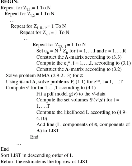
A summary of the estimation method is given in the form of pseudo-code in Fig. 2.

To initialize, choose the number of stepsN for discretizing the ½0;1 ranges of the uir. Let Zi;r be

integer variables. Set the all entries of matrix

U¼ fuirg to the value N1_{. Initialize LIST as an}

empty table with number of fields given by 1þRþIR, where 1accounts for the scalar value of L, R accounts for the components of p, andIRaccounts for the components ofA.

5.2. Fitting the pdf and computing volumes of polytopes

Since thevt_{-data lie in the interval ½0;1, a}

ver-satile pdf modeling approach can be based on the

two-parameter gamma pdf. First, transform the data by way of x¼ ðlnvÞ2 so that x2 ½0;1Þ. Then model the pdf of x as the two-parameter gamma pdf. Some related details can be found in Troutt et al. (2000), which provides a method of moments approach to fitting the gamma model.

For the evaluation of the volumes of the sets

St_ðvt_;xt_{Þ, which are convex polytopes, exact}

algo-rithms have been proposed. See, for example, B€ueler et al. (1998), Lawrence (1991), Verschelde et al. (1994), and Cohen and Hickey (1979). Codes in C are available through the home page website5 of Prof. K. Fukuda. In the numerical illustration that we present in the next section, the calculations are elementary and do not require the specialized software.

BEGIN:

Repeat for Z_1,1.= 1 To N Repeat for Z1,2.= 1 To N

…

Repeat for Z1, R−1.= 1 To N

Repeat for Z2,1 = 1 To N

…

Repeat for ZI,R−1 = 1 To N

Set uir= N −1_Z

irfor i = 1,…,I and r = 1,…,R

Construct the Λ-matrix according to (3.3)

Compute the κi*, i = 1,…,I, according to (3.1)

Construct the A-matrix according to (3.2)

Solve problem MMA (2.9-2.13) for π

Using ππand A, solve problems Pt(1.1) for zt*, t = 1,…,T

Compute vt_{for t = 1,…,T according to (4.1)}

Fit a pdf model g(v) to the vt_-data

Compute the set volumes St_(vt_,xt_{) for t =}

1,…,T

Compute the likelihood L according to (4.9-4.10)

Add line (L, components of π, components of

A) to LIST

End … End

Sort LIST in descending order of L Return the estimate as the top row of LIST

Fig. 2. Summary of the estimation procedure in pseudo-code form.

5.3. A numerical illustration on simulated data

An example of the procedure is developed here for simulated data. For simplicity, we consider two outputs and two inputs. In addition, constant input vectors are used. This permits an additional sim-plification in that problem MMA simplifies to an LP problem. This can be seen as follows. We have

xt_{¼ ðx}

1;x2Þ0 and nt¼ ðn1;n2Þ0 for all t. Then, in

problem MMA, the objective function simplifies to

max min

t p

0_yt_=nt0_xt

¼max min

t ðp1y t

1þp2y2tÞ=ðn1x1þn2x2Þ: ð5:1Þ

Now by the normalization constraint, n1x1þ

n2x2¼1, so that (5.1) simplifies further to

max mintp1y1tþp2y2t: ð5:2Þ

Objective functions of this kind can be converted to linear ones by the introduction of an auxiliary variable,w, for which

w¼min

t p1y t

1þp2y2t: ð5:3Þ

Then maximization ofw, along with the additional constraints

w6p1yt1þp2y2t for allt; ð5:4Þ

ensures that (5.3) holds at the optimal solution. Thus, it follows that problem MMA reduces to the following LP problem:

max w; ð5:5Þ

s:t: w6p1y1tþp2y2t for allt; ð5:6Þ

A0n¼p componentwise for allt; ð5:7Þ

p1yt1þp2y2t61for allt; ð5:8Þ

n1x1þn2x2¼1; ð5:9Þ

w;p1;p2;n1;n2P0: ð5:10Þ

Data sets consisting of 30 output vectors ðyt

1;y2tÞ,

t¼1;. . .;30, were simulated from the following stipulated true model:

Stipulated true LP model:

max p00y¼5y1þ3y2; ð5:11Þ

s:t: 2y1þy2640; ð5:12Þ

y1þ3y2660; ð5:13Þ

yiP0: ð5:14Þ

The constraints and objective function orientations for this model are depicted in Fig. 1. Thus, p0_{¼ ð5;3Þ}0_{, x}t_{¼ ð40;60Þ}0_{, and z}t _{¼108 for} t¼1;. . .;30. Random yt_{-observations were}

gen-erated as follows. First, a vt_{-value was simulated}

from the positive exponential density, gðvÞ ¼

gaðvÞ ¼Caeav,v2 ½0;1, for whichCa¼aðea1Þ

1

, and for which the cdf is given by GðvÞ ¼ ðea_1Þ1

ðeav_{1ÞThe parameter valuea¼8, was}

chosen. Then, for eachvt_{-value, ay}t_{such that}

po0_yt_¼vt_zt _ð5:15Þ

was generated using the uniform pdf on the line segment defined by the constraints (5.2)–(5.4) and (5.5). Fig. 1may be referenced again. The end-points of this segment were determined by maximizing and minimizing yt

2 subject to the feasibility constraints.

The Lebesgue measure of the set St_ðv;xt_{Þ is the}

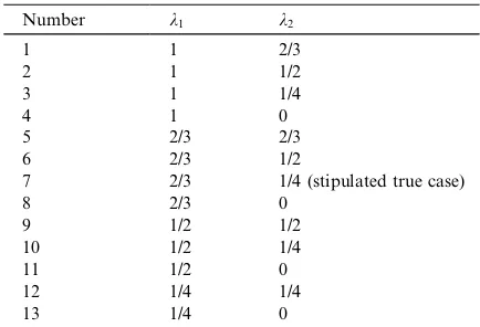
length of the line segment defined by those end-points, and the uniform pdf on the segment is the reciprocal of that length. Several candidate A -matrices were constructed as follows. Pairs of row generator vectors were selected as in Table 1. Then, the j_i-factors and corresponding A-matrices were computed according to the procedure of Section 3.

Twenty-five such data sets, of 30 observations each, were simulated and the estimation steps were completed for each data set. The estimatedp -vec-tor6 and the mean, v, of the vt_{-values were} Table 1

Candidate matrices

Number k1 k2

112/3

2 11/2

3 11/4

4 1 0

5 2/3 2/3

6 2/3 1/2

7 2/3 1/4 (stipulated true case)

8 2/3 0

9 1/2 1/2

10 1/2 1/4

11 1/2 0

12 1/4 1/4

13 1/4 0

obtained. The pdf modelgaðvÞ ¼Caeavwas fitted to the observedvt_{-values by the method of maximum}

likelihood estimation (MLE). The MLE estimate of

acan be verified to be the solution of the equation

a1ea_ðea_1Þ1

þv¼0; ð5:16Þ

which was solved by Newtons method using a starting value of a0¼2. Finally, the likelihood

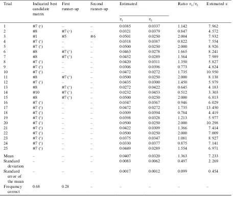
value for each observation was calculated using (4.9) and (4.10). The results were obtained using SAS/IML (1989) and are shown in Table 2.

From Table 2, the stipulated true matrix, number seven, was identified for 68% of these randomly simulated data sets. For those trials in which the maximum likelihood candidate was incorrect, the correct matrix was identified as having next highest likelihood in all but one trial. In addition, in all but one of the misidentified trials, matrix number eight was the one actually identified. It can be noted that matrix number eight is close to matrix number seven in the sense that one constraint is the same and the other has

Table 2

Estimation results for 25 consecutive data set simulations based on the stipulated assumptions

Trial Indicated best candidate matrix

First runner-up

Second runner-up

Estimated Ratiop1=p2 Estimateda

p1 p2

1#7 () – – 0.0385 0.0337 1.142 7.962

2 #8 #7 () – 0.03210.0379 0.847 4.572

3 #1#5 #6 0.05010.0250 2.004 7.932

4 #7 () – – 0.0318 0.0387 0.822 7.554

5 #7 () – – 0.0500 0.0250 2.000 8.926

6 #8 #7 () – 0.0463 0.0278 1.665 8.241

7 #8 #7 () – 0.0452 0.0289 1.564 7.989

8 #7 () – – 0.0420 0.0311 1.350 5.827

9 #7 () – – 0.0306 0.0396 0.773 4.824

1 0 #7 () – – 0.0472 0.0272 1.735 10.950

11 #8 #7 () – 0.0500 0.0250 2.000 8.138

1 2 #7 () – – 0.0435 0.0300 1.450 5.979

1 3 #8 #7 () – 0.0272 0.0422 0.645 4.183

1 4 #1 0 #7 () – 0.0232 0.0453 0.512 3.303

1 5 #8 #7 () – 0.0500 0.0250 2.000 6.813

1 6 #7 () – – 0.0347 0.0367 0.946 6.029

1 7 #7 () – – 0.0472 0.0272 1.735 13.450

1 8 #7 () – – 0.0309 0.0394 0.784 4.419

1 9 #7 () – – 0.0398 0.0328 1.213 5.977

20 #7 () – – 0.0500 0.0250 2.000 10.298

21#7 () – – 0.0422 0.0309 1.366 7.414

22 #7 () – – 0.0500 0.0250 2.000 7.009

23 #7 () – – 0.0375 0.0347 1.081 8.927

24 #7 () – – 0.0330 0.0377 0.875 7.141

25 #7 () – – 0.0449 0.0289 1.554 6.971

Mean – – – 0.0407 0.0320 1.363 7.233

Standard deviation

– – – 0.0083 0.0062 0.497 2.269

Standard error of the mean

– – – 0.0017 0.0012 0.099 0.454

Frequency correct

0.68 0.28 – – – – –

slope near to that of the other constraint of matrix number seven.

The mean of the estimated ratio p1=p2 was

1.363, as compared to 1.6, for the stipulated model. This is a difference of 2.39 standard errors of the mean. It should be noted that the stipulated model (5.11)–(5.14) has a large range of optimality that yields ratios in the range (0.333, 2.000). All trials but one, number three, yielded ratios in this range. Perhaps less estimation precision for the objective function vector should be expected due to the wide range of optimality for this example.

The reader is cautioned that these results are merely illustrative and do not constitute an ade-quate simulation study of the method. However, we believe they suggest that the method might be reasonably effective and is worthy of a more com-prehensive simulation study. For this example, the method appeared less effective in identifying the correct distribution parameter a. However, accu-racy of this estimate may be neither necessary nor sufficient for correct identification of the matrix. See, for example, trial nine (good matrix identifi-cation but poora-estimate) and trial three (gooda -estimate but poor matrix identification). Similar observations hold with respect to the a-estimate and thep1=p2ratio estimates. This is evidenced by

trials one, four, ten, eleven and fifteen in Table 2.

6. Limitations and potential extensions

6.1. Validation of the optimization goal

The major theoretical assumptions are that: (i) linear programming models with the samepandA

were appropriate for each observation, and (ii) that the organization or decision maker(s) have chosen or otherwise produced outputs which approximate optimal solutions to these models. The appropriateness of the second assumption can be judged to some degree by the magnitude of the likelihood scores, and the degree of concentration of the fitted gðvÞ pdf toward the ideal value of unity for v. In Troutt et al. (2000), a criterion, called normal-like-or-better performance effective-ness, has been proposed as a test for the optimi-zation goal.

6.2. Other decision model orientations

The basic decision model class assumed here is that of the Pt, which may be described as output-oriented. Namely, output values were to be approx-imately maximized subject to given resources. A cost minimization input-oriented model could be developed along similar lines. That is, suppose the data are regarded as attempts to minimize input costs subject to required outputs. The basic models,

Qt, analogous to thePt, can be given as

Qt: min n0xt_;

s:t: BxPyt; xP0; componentwise: ð6:1Þ

The model analogous to MMA can be easily constructed for this case.

Zeleny (1986) has called attention to the LP modeling flexibilities afforded by regarding re-source levels as additional decision variables in what are called De Novo LP models. Such con-structs adapted to the present setting clearly pro-vide an avenue for further research on mixed input–output orientations.

6.3. The unbounded pdf heuristic

For the positive exponential gðvÞthat we used for the numerical illustration, the pdf value at the upper end-point of the interval gð1Þ is bounded and greater than zero. If yt_¼yt _{and y}t _{is the}

unique optimal solution of problem Pt, then

mðSt_ðv;xt_{ÞÞ ¼0 in (4.9), and thus (4.9) tends to the}

Other heuristics could be proposed. For exam-ple, the xt_{-vectors might be stretched by a factor}

such as 1þein order to prevent any data vector,

yt_{, from being an exactly optimal solution to its}

respective problemPt. However, we have not ob-served the occurrence of these problem cases so far in our experiments with the method.

6.4. Use of other aggregators in the MDE technique

The sum or average aggregator could be used to develop a model like the MMA model above. The resulting model would require maximization of the sum of the efficiency ratios. While the problem of optimizing the sum of linear fractional functions subject to linear constraints is challenging, some algorithms have been proposed. Schaible and Shi (2003) provide a recent survey.

7. Conclusions

We have defined a version of the Inverse LP problem that we call Linear Programming System Identification. This problem seeks to identify both the objective function coefficient vector and the constraint matrix of a linear programming prob-lem that best fits a set of observed vector pairs. One vector of each pair is considered an approxi-mately optimal decision vector for the linear pro-gramming problem when the other vector is the resource vector of that problem. An algorithm was proposed for approximating a maximum likeli-hood solution. Results were illustrated for an example in two dimensions. Some preliminary simulation results for that example suggest that the method may be promising and is worthy of a more comprehensive simulation study for future re-search.

Acknowledgements

We wish to thank an anonymous referee for many helpful suggestions. We are also indebted to Dr. L.F. Cheung for stimulating discussions.

References

Ahuja, R.K., Orlin, J.B., 2001. Inverse optimization. Opera-tions Research 49 (5), 771–783.

Barros, A.I., Frenk, J.B.G., Schaible, S., Zhang, S., 1996a. A new algorithm for generalized fractional programs. Math-ematical Programming 72, 147–175.

Barros, A.I., Frenk, J.B.G., Schaible, S., Zhang, S., 1996b. Using duality to solve generalized fractional programming problems. Journal of Global Optimization 8, 139–170. B€ueler, B., Enge, A., Fukuda, K., 1998. Exact volume

compu-tation for convex polytopes a practical study. In: Kalai, G., Ziegler, G. (Eds.), Polytopes––Combinatorics and Compu-tation. DMV-Seminars. Birkh€auser Verlag.

Cohen, J., Hickey, T., 1979. Two algorithms for determining volumes of convex polyhedra. Journal of the Association for Computing Machinery 26 (3), 401–414.

Crouzeix, J.J., Ferland, J.A., 1991. Algorithms for generalized fractional programming. Mathematical Programming 52, 191–207.

Crouzeix, J.J., Ferland, J.A., Schaible, S., 1985. An algorithm for generalized fractional programs. Journal of Optimiza-tion Theory and ApplicaOptimiza-tions 47, 35–49.

Gugat, M., 1996. A fast algorithm for a class of generalized fractional programs. Management Science 42 (10), 1493– 1499.

Lawrence, J., 1991. Polytope volume computation. Mathemat-ics of Computation 57 (196), 259–271.

Pardalos, P.U., Phillips, A.T., 1991. Global optimization of fractional programs. Journal of Global Optimization 1, 173–182.

SAS/IML, 1989. Software: Usage and Reference. Version 6, first ed. SAS Institute, Inc., Cary, NC.

Schaible, S., Shi, J., 2003. Fractional programming: The sum-of-ratios case. Optimization Methods and Software 18 (2), 219–229.

Tarantola, A., 1987. Inverse Problem Theory: Methods for Data Fitting and Model Parameter Estimation. Elsevier, Amsterdam.

Troutt, M.D., 1995. A maximum decisional efficiency estima-tion principle. Management Science 41, 76–82.

Troutt, M.D., Gribbin, D.W., Shanker, M., Zhang, A., 2000. Cost efficiency benchmarking for operational units with multiple cost drivers. Decision Sciences 31(4), 813–832. Troutt, M.D., Pang, W.-K., Hou, S.-H., 2003. Vertical Density

Representation and Its Applications. World Scientific Pub-lishing Co. Pte. Ltd., Singapore.

Verschelde, J., Verlinden, P., Cools, R., 1994. Homotopies exploiting Newton polytopes for solving sparse polynomial systems. SIAM Journal on Numerical Analysis 31(3), 915– 930.

Zhang, J., Liu, Z., 1996. Calculating some inverse linear programming problems. Journal of Computational and Applied Mathematics 72, 261–273.