Institut Teknologi Nasional Januari – Maret 2010
An Application of the Multi-Level Heuristic for the
Heterogeneous Fleet Vehicle Routing Problem
ARIF IMRAN
Department of Industrial Engineering, Institut Teknologi Nasional Bandung Email: [email protected]
ABSTRACT
The Multi-Level heuristic is used to investigate the heterogeneous fleet vehicle routing problem (HFVRP). The initial solution for the Multi-Level heuristic is obtained by Dijkstra’s algorithm based on a cost network constructed by the sweep algorithm and the 2-opt procedure. The proposed algorithm uses a number of local search operators such as swap, 1-0 insertion, 2-opt, and Dijkstra’s Algorithm. In addition, in order to improve the search process, a diversification procedure is applied. The proposed algorithm is then tested on the data sets from the literature.
Keywords: multi-level, heuristic, routing, heterogeneous fleet
ABSTRAK
Algoritma Multi-Level heuristic digunakan untuk melakukan investigasi terhadap heterogeneous fleet vehicle routing problem (HFVRP). Solusi inisial Multi-Level heuristic didapatkan dari algoritma Dijkstra berdasarkan cost network yang dibentuk oleh agoritma sweep dan prosedur 2-opt. Algoritma Multi-Level heuristic yang dikembangkan memakai sejumlah operator local search seperti, swap, 1-0 insertion, 2-opt, and algoritma Dijkstra. Untuk memperbaiki proses pencarian solusi (search process) satu prosedur diversifikasi juga diaplikasikan. Selanjutnya, algoritma yang dikembangkan diuji untuk menyelesaikan data-data yang terdapat pada literatur.
1. INTRODUCTION
The heterogeneous fleet vehicle routing problem is a variant of the vehicle routing problem (VRP) where the vehicles do not necessary have the same capacity, vehicle fixed cost, and unit variable cost. We are also given a set of customers, N, a certain number of vehicle types, M, each of which has a vehicle capacity Qm, a fixed cost Fm and a unit variable cost Rm (m = 1,…,M). As in the classical VRP, each customer must be served by one vehicle only, each vehicle must start and finish its journey at a central depot and the capacity of a vehicle and the maximum length of a route must not be exceeded. The objective of the heterogeneous fleet vehicle routing problem (HFVRP) is to minimize the total cost which includes both the vehicle variable and fixed costs. The idea is not only to consider the routing of the vehicles, but also the composition of the vehicle fleet.
There are a number of published papers addressing the HFVRP. Golden et al. [10] were among the first authors to tackle this problem using a constant unit variable cost. They developed algorithms based on the Clarke and Wright [4] saving technique for the VRP as well as two implementations of the giant tour based algorithm. Salhi and Rand [19] put forward an interactive route perturbation procedure (RPERT) which contains seven refinement phases, each aimed at constructing a newly constructed fleet with a lower total cost. Osman and Salhi [15] proposed two algorithms; the first one based on a tabu search and the second is a modification of RPERT. Ochi et al. [14] presented an evolutionary hybrid metaheuristic which combines a parallel genetic algorithm with scatter search. Gendreau et al. [8] implemented a tabu search approach using GENIUS, initially developed by Gendreau et al. [6] for the TSP, and some search strategies from Gendreau et al. [7] as well as the adaptive memory procedure originally developed for the VRP by Rochat and Taillard [17]. Taillard [22] presented a heuristic using a column generation method. Renaud and Boctor [16] proposed a sweep-based algorithm to generate a large set of good routes, which are then used in a set partitioning algorithm. Wassan and Osman [23] developed tabu search variants including reactive tabu search that uses special data memory structures and hashing functions. Yaman [24] put forward six formulations for the HFVRP. The first four formulations are based on Miller-Tucker-Zemlin constraints whereas the last two, which proved to be more successful, use flow variables. Choi and Tcha [3] used an application of column generation technique which is enhanced by dynamic programming schemes. Lee et al. [12] put forward an algorithm that uses tabu search and set partitioning. More recently, Brandao [2] developed two variants of the deterministic tabu search algorithm and Imran et al. [11] put forward an adaptation of the VNS algorithm, which produce excellent results when tested to three data sets from the literature.
The remaining parts of the paper are organized as follows: section two presents the proposed Multi Level algorithm is presented; section three provides the explanation of its main steps; section four gives the computational results; and the last section summarizes our findings.
2. THE MULTI LEVEL HEURISTIC
Figure 1. The Multi-Level-Based Algorithm
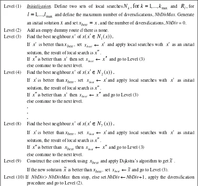
In level 1, the initial solution is generated using the adapted sweep for the VRP and Dijkstra’s algorithm for the HFVRP. Level (2) functions as a generator of the empty route. In Level (3) to Level (8), six refinement procedures (neighborhood) are used, namely 1-1 interchange, 2-0 shift of type 1, 2-1 interchange, perturbation of type 1, perturbation of type 2, and 2-0 shift of type 2, respectively. After the refinement procedures (neighborhood) mentioned above are performed, we implement, in each level, starting from Level (3) to Level (8), two types of local search procedures namely the intra-route and the inter-route. Intra-route procedures consist of the 1-0 insertion route, 2-0 insertion route, the swap and the 2-opt intra-route. Meanwhile, route procedures consist of the 1-0 interchange and the 2-opt inter-route. A multi-level approach is also used for both intra and inter-route refinement procedures. In Level (9) Dijkstra’s algorithm is applied, if no better solution is found in Level (8). If Dijkstra’s algorithm cannot improve the solution, Level (10), the diversification procedure is utilised and the search reverts to level 2.
Level (1) Initialization. Define two sets of local searches
N
k,
for
k
1
,...,
k
max andR
l,
for max,...,
1
l
l
and define the maximum number of diversifications, NbDivMax. Generate an initial solutionx
and setx
best
x
, and the number of diversifications, NbDiv = 0. Level (2) Add an empty dummy route if there is none.Level (3) Find the best neighbour
x
'
ofx(xN1(x)).If
x
'
isbetter thanx
best, set xbest x
'
and apply local searches withx
'
as an initialsolution, the result of local search is
x
.If
x
is better thanx
'
thenset xbest x
and go to Level (3) elsecontinueto the next level.Level (4) Find the best neighbour
x
'
ofx(xN2(x)).If
x
'
is better thanx
best, set xbest x
'
and apply local searches withx
'
as initial solution, the result of local search isx
.If
x
is better thanx
'
then xbest x
and go to Level (3) elsecontinueto the next level.. . .
Level (8) Find the best neighbour
x
'
ofx
(
x
N
7(
x
))
.If
x
'
is better thanx
best, set xbest x
'
and apply local searches withx
'
as initial solution, the result of local search isx
.If
x
is better thanx
best then xbest x
and go to Level (3)elsecontinueto the next level.
Level (9) Construct the cost network using
x
best and apply Dijkstra’s algorithm to getx
~
. If the new solutionx
~
is better thanx
best, set xbest~xand go to Level (3).3. EXPLANATION OF MAIN STEPS
3.1 Initial solution
The initial solution is obtained in three steps: (a) construct a giant tour using the sweep algorithm of Gillett and Miller [9], (b) improve this tour using the 2-opt of Lin [13], and (c) construct the cost network and then apply Dijkstra’s algorithm [5] to find the corresponding optimal fleet size. Dijkstra’s algorithm systematically provides an initial solution that contains routes with their appropriate types of vehicles. This partitioning procedure based on solving the shortest path problem was presented by Beasley [1] for solving the VRP and by Golden et al. [10] for the HFVRP. To avoid using the largest distance between two successive customers in a given route, the starting points, in the construction of the cost network, are used as those that generate the highest largest distances between two successive customers (i.e. gaps) in the giant tour. The number of gaps (NG) generated is defined as follows:
NG= ))}
where NR is the number of routes found by Dijkstra’s algorithm, (i,i+1) the ordered sequence of customers,
g
ithe ith gap (i.e. the distance between customer i and i+1), g the average gap, andg
the largest gap. The reasoning of using (1) is based on the idea of linking the value of NG to the number of routes and also to the number of gaps that relate to the average as well as the largest gap. For each of the NG selected gaps, say (i1,i1+1), two cost networks are then generated starting from i1anticlockwise and from i1+1 clockwise. Dijkstra’s algorithm is then applied to each of these
2
NG
cost networks. The complete explanation to obtain the initial solution can be found in Imran et al. [11].
Adding flexibility via an empty dummy route
In this step, a procedure is used to create an empty route after the initialization phase and also when the diversification procedure is applied. Note that in the search we only need one empty route in the system at any time. In the case a second empty route materializes during the search, we systematically remove it. The empty route provides the search with extra flexibility as this may reduce the total cost if found worthwhile by allowing the load served from a large vehicle to be split into two smaller vehicles.
3.2 Neighborhood Structures
Six neighborhoods, which are briefly described in this subsection, are used in this study (i.e. kmax = 6).
These include the 1-1 interchange (swap), two types of the 2-0 shift, the 2-1 interchange, and two types of the perturbation. The order of the neighborhoods is as follows; the 1-1 interchange is used as N1, the 2-0 shift of type 1 as N2, the 2-1 interchange as N3, the perturbation of type 1 as N4, the
perturbation of type 2 as N5, and finally the 2-0 shift of type 2 as N6.
The 1-1 interchange (the swap procedure)
This neighborhood is aimed at generating a feasible solution by swapping a pair of customers from two routes. This procedure starts by taking a random customer from a randomly chosen route and tries to swap it systematically with other customers by taking into consideration all other routes. This procedure is repeated until a feasible move is found.
The 2-0 shift
The 2-1 interchange
This type of insertion attempts to shift two consecutive random customers from a randomly chosen route to another route selected systematically while getting one customer from the receiver route until a feasible move is obtained.
A new perturbation mechanism
This scheme was initially developed by Salhi and Rand [18] for the VRP by considering three routes simultaneously. Here, it starts by taking a random customer from a randomly chosen route and tries to relocate that customer into another route without considering capacity and time constraints in the receiver route. A customer from the receiver route is then shifted to the third route if both capacity and time constraints for the second and the third route are not violated. We refer to this as the perturbation of type 1. An extension of such a perturbation is the one that shifts two consecutive customers from a route. In this procedure, instead of removing one customer at the beginning we remove two customers. We name this procedure as the perturbation of type 2.
3.3 Local Search
Local searches used in this work are the 1-insertion intra-route, 2-insertion intra-route, 1-1 interchange intra-route, the 2-opt intra-route, the 1-insertion inter-route and 2-opt inter-route.
The 1-1 interchange (inter-route and intra-route)
The swap intra-route is aimed at reducing the total cost of a route by swapping positions of a pair of customers within the route. Meanwhile the intra-route one reducing the total cost by by swapping positions of a pair of customers from different route.
The 1-insertion procedures (inter-route and intra-route)
Two types of the 1-insertion procedures are used. The first is the 1-insertion intra-route and the second is the 1-insertion inter-route. In the 1-insertion intra-route we remove a customer from its position in a route and try to insert it elsewhere within that route in order to have a better solution. Meanwhile, in the 1-insertion inter-route, each customer from a route is shifted from its position and tried to be inserted elsewhere into another route. If this shifting does not violate any constraints and improves the solution, the selected customer is then permanently removed.
The 2-insertion (intra-route)
The 2-insertion intra-route allows us to remove two consecutive customers and insert them elsewhere within a route to produce a cheaper route.
The 2-opt (inter-route and intra-route)
The 2-opt intra-route, usually refer to as the 2-opt (see Lin [13]), works by removing two non adjacent arcs and adding two new arcs while maintaining the tour structure. A given exchange is accepted if the resulting total cost is lower than the previous total cost. The exchange process is continued until no further improvement can be found. The 2-opt inter-route is similar to the 2-opt intra-route except that it considers two routes where each of the two arcs belong to a different route and reverse directions of the corresponding affected path of each route.
3.4 Use of Dijkstra’s Algorithm as an Extra Refinement
tour. The steps of this procedure, when the first point of the first route is used to construct a network, are presented in Figure 2.
Figure 2. Construction of the cost network
When we start from the other end point (i.e., the last node) of the first route, the order of that route is reversed but step 2 and step 3 of Figure 3 are similar. This construction obviously ensures that the current solution is feasible and hence Dijkstra’s algorithm might discover a better one.
The Diversification Procedure (Step 5)
This procedure is used when there is no further improvement after all the local searches are performed. The idea is to explore other regions of the search space that may not have been visited otherwise. The incumbent best solution is used as an input for the diversification procedure to obtain the new initial solution. The idea is to construct a cost network by starting from a node which is not the first point of any route, when following clockwise direction, and also not the end point of any route, when following anticlockwise direction. This will ensure that a route from this incumbent best solution will be split, a new cost network constructed and hence a new solution generated. The steps of the diversification procedure are presented in Figure 3. In this study, the number of diversifications (ND)
is set asNDMin(100 ,2N), where N represents the number of customers in a given instance.
Figure 3: The diversification procedure
4. COMPUTATIONAL EXPERIENCE
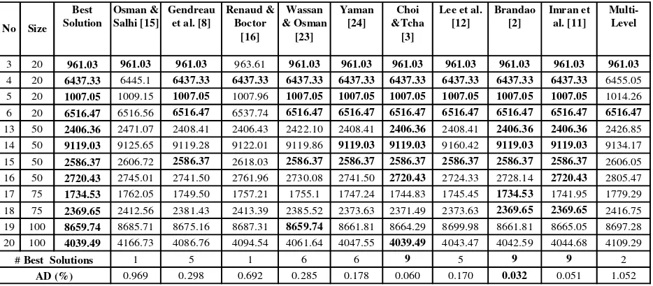
The Multi-Level based heuristic is programmed in C++ and executed on a Pentium IV 2.4 GHz PC with 512 MB RAM. The algorithm is tested on the Golden et al. [10] data set. For comparison, we present the best results found by several authors. For each instance, say k, we compute the relative percentage deviation as
(cos
t
k
best
k)
best
k
100
,
where costk and bestk denote, for the kthinstance, the cost found by our heuristic and the best known solution respectively. The average deviation (AD) is then computed over all instances. Table 1 show that our algorithm produces two solutions, instance #3 and instance #4, which are similar to the best known solutions. The Average Deviation obtained is nearly as good as the one of Osman and Salhi [15]. In terms of the CPU time, our algorithm is fast as can be seen in Table 2. The comparison of the CPU time with the previous research is given in Table 2.
Step 1. Use the first node of the first route as the starting point.
Step 2. Connect the nearest end points of other routes with the last node of the first route. Select the route which has the nearest end point as the next route. If the nearest end point is the last point in that route, reverse the route order.
Step 3. Apply Step 2 to the remaining routes by starting from the selected route in Step 2.
Step 1. Connect all points; the last point of the previous route is connected to the first point of the next route.
Step 2. Calculate all distances between two consecutive points.
Step 3. Select the largest distance between two consecutive points which are not two end points of different routes, say as the starting point.
Step 4. Construct the cost network starting (e1,e2)from e2clockwise and apply the Dijkstra’s Algorithm.
Table 1. Solution Quality from the Different Methods
3 20 961.03 961.03 963.61 961.03 961.03 961.03 961.03 961.03 961.03 961.03 4 20 6445.1 6437.33 6437.33 6437.33 6437.33 6437.33 6437.33 6437.33 6437.33 6455.05 5 20 1009.15 1007.05 1007.96 1007.05 1007.05 1007.05 1007.05 1007.05 1007.05 1014.26 6 20 6516.56 6516.47 6537.74 6516.47 6516.47 6516.47 6516.47 6516.47 6516.47 6516.47 13 50 2471.07 2408.41 2406.43 2422.10 2408.41 2406.36 2408.41 2406.36 2406.36 2426.85 14 50 9125.65 9119.28 9122.01 9119.86 9119.03 9119.03 9160.42 9119.03 9119.03 9134.17 15 50 2606.72 2586.37 2618.03 2586.37 2586.37 2586.37 2586.37 2586.37 2586.37 2606.05 16 50 2745.01 2741.50 2761.96 2730.08 2741.50 2720.43 2724.33 2728.14 2720.43 2805.47 17 75 1762.05 1749.50 1757.21 1755.1 1747.24 1744.83 1745.45 1734.53 1741.95 1779.29 18 75 2412.56 2381.43 2413.39 2385.52 2373.63 2371.49 2373.63 2369.65 2369.65 2416.75 19 100 8685.71 8675.16 8687.31 8659.74 8661.81 8664.29 8699.98 8661.81 8665.05 8697.28 20 100 4166.73 4086.76 4094.54 4061.64 4047.55 4039.49 4043.47 4042.59 4044.68 4109.29
1 5 1 6 6 9 5 9 9 2
0.969 0.298 0.692 0.285 0.178 0.060 0.170 0.032 0.051 1.052
Multi-Table 2. CPU Time Comparison (in Seconds) for the HFVRP
No Size Taillard
REFERENCES
[1] Beasley, J., (1983). “Route First-Cluster Second Methods for Vehicle Routing”. Omega, 11, 403-408.
[2] Brandao, J., (2009). “A Deterministic Tabu Search Algorithm for the Fleet Size and Mix Vehicle Routing Problem”. European Journal of Operational Research,195, 716-728.
[3] Choi, E., Tcha D.-W., (2007). “A Column Generation Approach to the Heterogeneous Fleet Vehicle Routing Problem”. European Journal of Operational Research, 34,2080-2095. [4] Clarke, G. dan Wright, J.W., (1964). “Scheduling of Vehicle from Central Depot to a Number of
Delivery Points”. Operations Research, 12,568-581.
[5] Dijkstra, E.W., (1959). “A Note on Two Problems in Connection with Graphs”. Numerische Mathematik,1, 269-271.
[6] Gendreau, M., Hertz, A., dan Laporte, G., (1992). “New Insertion and Post Optimization Procedures for the Traveling Salesman Problem”. Operations Research, 40,1086-1094.
[7] Gendreau, M., Hertz, A., dan Laporte, G., (1994). “A Tabu Search Algorithm for the Vehicle Routing Problem”. Management Science,40,1276-1290.
[8] Gendreau, M., Laporte, G., Musaraganyi, C., dan Taillard, E.D., (1999). “A Tabu Search Heuristic for the Heterogeneous Fleet Vehicle Routing Problem”. Computers & Operations Research, 26, 1153-1173.
[9] Gillett, B.E. dan Miller, L.R., (1974). ”A Heuristic Algorithm for the Vehicle Dispatch Problem”. Operations Research,22,340-344.
[10] Golden, B., Assad, A., Levy, L., dan Gheysens, F., (1984). “The Fleet Size and Mix Vehicle Routing”. Computers & Operations Research, 11,49-66.
[11] Imran, A., Salhi, S. dan Wassan N.A. (2009). “A Variable Neighborhood-Based Heuristic for the Heterogeneous Fleet Vehicle Routing Problem”. European Journal of Operational Research, 197, 509-518.
[12] Lee,Y.H., Kim, J.I., Kang, K.H., dan Kim, K.H., (2008). “A Heuristic for Vehicle Fleet Mix Problem Using Tabu Search and Set Partitioning”. Journal of the Operational Research Society, 59,833-841.
[13] Lin, S., (1965). “Computers Solutions of the Traveling Salesman Problem”. Bell System Technical Journal, 44,2245-2269.
[14] Ochi, L.S., Viana D.S., Drummond L.M.A., dan Victor A.O., (1998). “A parallel Evolutionary Algorithm for the Vehicle Routing Problem with Heterogeneous Fleet”. Future Generation Computation System, 14, 285-292.
[15] Osman, I.H. dan Salhi, S., 1996. Local Search Strategies for the Mix Fleet Routing Problem. In: Rayward-Smith, V.J., Osman, I.H., Reeves, C.R., Smith, G.D. (Eds.), Modern Heuristic Search Methods, pages 132-153. John Wiley & Sons.
[16] Renaud, J., dan Boctor, F.F., (2002). “A Sweep-Based Algorithm for the Fleet Size and Mix Vehicle Routing Problem”. European Journal of Operational Research, 140,618-628.
[17] Rochat, Y. dan Taillard, E.D., (1995). “Probabilistic Diversification and Intensification in Local Search Vehicle Routing”. Journal of Heuristic, 1,147-167.
[18] Salhi, S., Rand, G.K., (1987). “Improvements to Vehicle Routing Heuristics”. Journal of the Operational Research Society,38,293-295.
[19] Salhi, S. dan Rand, G.K., (1993). “Incorporating Vehicle Routing into the Vehicle Fleet Composition Problem”. European Journal of Operational Research, 66,313-360.
[20] Salhi, S. dan Sari, M., (1997). “A Multi-Level Composite Heuristic for the Multi-Depot Vehicle Fleet Mix Problem”. European Journal of Operational Research, 103,95-112.
[21] Salhi, S., Sari, M., Sadi, D., dan Touati, N., (1992). “Adaptation of Some Vehicle Fleet Mix Heuristic”. OMEGA,20,653-660.
[22] Taillard, E.D., (1999). “A Heuristic Column Generation Method for the Heterogeneous Fleet VRP”. Recherche Operationnelle, 33,1-14.
[23] Wassan, N.A. dan Osman, I.H., (2002). “Tabu Search Variants for the Mix Fleet Vehicle Routing Problem”. Journal of the Operational Research Society,53,768-782.