A Pr actical Appr oac h to Design, Implementation, and Manag ement

(1)

Connoll

y • Begg

GloBal

EDITION

Glo

B

al

title widely used by colleges and universities throughout the world. Pearson published this exclusive edition for the benefit of students outside the United States and Canada. If you purchased this book within the United States or Canada you should be aware that it has been imported without the approval of the Publisher or author.

GloBal

For these Global Editions, the editorial team at Pearson has

collaborated with educators across the world to address a

wide range of subjects and requirements, equipping students

with the best possible learning tools. This Global Edition

preserves the cutting-edge approach and pedagogy of the

original, but also features alterations, customization and

adaptation from the North american version.

Database Systems

A Practical Approach to Design, Implementation,

and Management

SIXTH EDITION

(2)

6

SQL: Data Manipulation

Chapter Objectives

In this chapter you will learn:

• The purpose and importance of the Structured Query Language (SQL). • The history and development of SQL.

• How to write an SQL command.

• How to retrieve data from the database using the SELECT statement. • How to build SQL statements that:

– use the WHERE clause to retrieve rows that satisfy various conditions;

– sort query results using ORDER BY;

– use the aggregate functions of SQL;

– group data using GROUP BY;

– use subqueries;

– join tables together;

– perform set operations (UNION, INTERSECT, EXCEPT).

• How to perform database updates using INSERT, UPDATE, and DELETE.

In Chapters 4 and 5 we described the relational data model and relational lan-guages in some detail. A particular language that has emerged from the develop-ment of the relational model is the Structured Query Language, or SQL as it is commonly called. Over the last few years, SQL has become the standard relational database language. In 1986, a standard for SQL was defined by the American National Standards Institute (ANSI) and was subsequently adopted in 1987 as an international standard by the International Organization for Standardization (ISO, 1987). More than one hundred DBMSs now support SQL, running on vari-ous hardware platforms from PCs to mainframes.

Owing to the current importance of SQL, we devote four chapters and an appendix of this book to examining the language in detail, providing a com-prehensive treatment for both technical and nontechnical users including pro-grammers, database professionals, and managers. In these chapters we largely

(3)

concentrate on the ISO definition of the SQL language. However, owing to the complexity of this standard, we do not attempt to cover all parts of the language. In this chapter, we focus on the data manipulation statements of the language.

Structure of this Chapter

In Section 6.1 we introduce SQL and discuss why the language is so important to database applications. In Section 6.2 we introduce the notation used in this book to specify the structure of an SQL state-ment. In Section 6.3 we discuss how to retrieve data from relations using SQL, and how to insert, update, and delete data from relations.

Looking ahead, in Chapter 7 we examine other features of the language, including data definition, views, transactions, and access control. In Chapter 8 we examine more advanced features of the language, including triggers and stored procedures. In Chapter 9 we examine in some detail the features that have been added to the SQL specification to support object-oriented data management. In Appendix I we discuss how SQL can be embedded in high-level programming languages to access constructs that were not available in SQL until very recently. The two formal languages, relational algebra and relational calculus, that we covered in Chapter 5 provide a foundation for a large part of the SQL standard and it may be useful to refer to this chapter occasionally to see the similarities. However, our presentation of SQL is mainly independent of these languages for those readers who have omitted Chapter 5. The examples in this chapter use the

DreamHome rental database instance shown in Figure 4.3.

6.1 Introduction to SQL

In this section we outline the objectives of SQL, provide a short history of the lan-guage, and discuss why the language is so important to database applications.

6.1.1 Objectives of SQL

Ideally, a database language should allow a user to:

• create the database and relation structures;

• perform basic data management tasks, such as the insertion, modification, and deletion of data from the relations;

• perform both simple and complex queries.

A database language must perform these tasks with minimal user effort, and its command structure and syntax must be relatively easy to learn. Finally, the lan-guage must be portable; that is, it must conform to some recognized standard so that we can use the same command structure and syntax when we move from one DBMS to another. SQL is intended to satisfy these requirements.

(4)

• a Data Definition Language (DDL) for defining the database structure and con-trolling access to the data;

• a Data Manipulation Language (DML) for retrieving and updating data.

Until the 1999 release of the standard, known as SQL:1999 or SQL3, SQL con-tained only these definitional and manipulative commands; it did not contain flow of control commands, such as IF . . . THEN . . . ELSE, GO TO, or DO . . . WHILE. These commands had to be implemented using a programming or job-control language, or interactively by the decisions of the user. Owing to this lack of

computational completeness, SQL can be used in two ways. The first way is to use SQL

interactively by entering the statements at a terminal. The second way is to embed

SQL statements in a procedural language, as we discuss in Appendix I. We also discuss the latest release of the standard, SQL:2011 in Chapter 9.

SQL is a relatively easy language to learn:

• It is a nonprocedural language; you specify what information you require, rather than how to get it. In other words, SQL does not require you to specify the access methods to the data.

• Like most modern languages, SQL is essentially free-format, which means that parts of statements do not have to be typed at particular locations on the screen. • The command structure consists of standard English words such as CREATE

TABLE, INSERT, SELECT. For example:

– CREATE TABLE Staff (staffNo VARCHAR(5), IName VARCHAR(15), salary

DECIMAL(7,2));

– INSERT INTOStaffVALUES (‘SG16’, ‘Brown’, 8300); – SELECTstaffNo, IName, salary

FROMStaff

WHEREsalary > 10000;

• SQL can be used by a range of users including database administrators (DBA), management personnel, application developers, and many other types of end-user.

An international standard now .exists for the SQL language making it both the formal and de facto standard language for defining and manipulating relational databases (ISO, 1992, 2011a).

6.1.2 History of SQL

As stated in Chapter 4, the history of the relational model (and indirectly SQL) started with the publication of the seminal paper by E. F. Codd, written during his work at IBM’s Research Laboratory in San José (Codd, 1970). In 1974, D. Chamberlin, also from the IBM San José Laboratory, defined a language called the Structured English Query Language, or SEQUEL. A revised version, SEQUEL/2, was defined in 1976, but the name was subsequently changed to SQL for legal rea-sons (Chamberlin and Boyce, 1974; Chamberlin et al., 1976). Today, many people still pronounce SQL as “See-Quel,” though the official pronunciation is “S-Q-L.”

IBM produced a prototype DBMS based on SEQUEL/2 called System R (Astrahan

(5)

SQL are in the language SQUARE (Specifying Queries As Relational Expressions), which predates the System R project. SQUARE was designed as a research language to implement relational algebra with English sentences (Boyce et al., 1975).

In the late 1970s, the database system Oracle was produced by what is now called the Oracle Corporation, and was probably the first commercial implementation of a relational DBMS based on SQL. INGRES followed shortly afterwards, with a query language called QUEL, which although more “structured” than SQL, was less English-like. When SQL emerged as the standard database language for rela-tional systems, INGRES was converted to an SQL-based DBMS. IBM produced its first commercial RDBMS, called SQL/DS, for the DOS/VSE and VM/CMS envi-ronments in 1981 and 1982, respectively, and subsequently as DB2 for the MVS environment in 1983.

In 1982, ANSI began work on a Relational Database Language (RDL) based on a concept paper from IBM. ISO joined in this work in 1983, and together they defined a standard for SQL. (The name RDL was dropped in 1984, and the draft standard reverted to a form that was more like the existing implementations of SQL.)

The initial ISO standard published in 1987 attracted a considerable degree of criticism. Date, an influential researcher in this area, claimed that important features such as referential integrity constraints and certain relational operators had been omitted. He also pointed out that the language was extremely redundant; in other words, there was more than one way to write the same query (Date, 1986, 1987a, 1990). Much of the criticism was valid, and had been recognized by the standards bodies before the standard was published. It was decided, however, that it was more important to release a standard as early as possible to establish a common base from which the language and the implementations could develop than to wait until all the features that people felt should be present could be defined and agreed.

In 1989, ISO published an addendum that defined an “Integrity Enhancement Feature” (ISO, 1989). In 1992, the first major revision to the ISO standard occurred, sometimes referred to as SQL2 or SQL-92 (ISO, 1992). Although some features had been defined in the standard for the first time, many of these had already been implemented in part or in a similar form in one or more of the many SQL implementations. It was not until 1999 that the next release of the standard, commonly referred to as SQL:1999 (ISO, 1999a), was formalized. This release contains additional features to support object-oriented data management, which we examine in Chapter 9. There have been further releases of the standard in late 2003 (SQL:2003), in summer 2008 (SQL:2008), and in late 2011 (SQL:2011).

Features that are provided on top of the standard by the vendors are called

extensions. For example, the standard specifies six different data types for data in an SQL database. Many implementations supplement this list with a variety of extensions. Each implementation of SQL is called a dialect. No two dialects are exactly alike, and currently no dialect exactly matches the ISO standard. Moreover, as database vendors introduce new functionality, they are expanding their SQL dialects and moving them even further apart. However, the central core of the SQL language is showing signs of becoming more standardized. In fact, SQL now has a set of features called Core SQL that a vendor must implement to claim

(6)

Although SQL was originally an IBM concept, its importance soon motivated other vendors to create their own implementations. Today there are literally hundreds of SQL-based products available, with new products being introduced regularly.

6.1.3 Importance of SQL

SQL is the first and, so far, only standard database language to gain wide accept-ance. The only other standard database language, the Network Database Language (NDL), based on the CODASYL network model, has few followers. Nearly every major current vendor provides database products based on SQL or with an SQL interface, and most are represented on at least one of the standard-making bodies. There is a huge investment in the SQL language both by vendors and by users. It has become part of application architectures such as IBM’s Systems Application Architecture (SAA) and is the strategic choice of many large and influential organi-zations, for example, the Open Group consortium for UNIX standards. SQL has also become a Federal Information Processing Standard (FIPS) to which conform-ance is required for all sales of DBMSs to the U.S. government. The SQL Access Group, a consortium of vendors, defined a set of enhancements to SQL that would support interoperability across disparate systems.

SQL is used in other standards and even influences the development of other standards as a definitional tool. Examples include ISO’s Information Resource Dictionary System (IRDS) standard and Remote Data Access (RDA) standard. The development of the language is supported by considerable academic interest, providing both a theoretical basis for the language and the techniques needed to implement it successfully. This is especially true in query optimization, distribution of data, and security. There are now specialized implementations of SQL that are directed at new markets, such as OnLine Analytical Processing (OLAP).

6.1.4 Terminology

The ISO SQL standard does not use the formal terms of relations, attributes, and tuples, instead using the terms tables, columns, and rows. In our presentation of SQL we mostly use the ISO terminology. It should also be noted that SQL does not adhere strictly to the definition of the relational model described in Chapter 4. For example, SQL allows the table produced as the result of the SELECT statement to contain duplicate rows, it imposes an ordering on the columns, and it allows the user to order the rows of a result table.

6.2 Writing SQL Commands

In this section we briefly describe the structure of an SQL statement and the nota-tion we use to define the format of the various SQL constructs. An SQL statement consists of reserved words and user-defined words. Reserved words are a fixed part of the SQL language and have a fixed meaning. They must be spelled exactly

(7)

does not require it, many dialects of SQL require the use of a statement terminator to mark the end of each SQL statement (usually the semicolon “;” is used).

Most components of an SQL statement are case-insensitive, which means that letters can be typed in either upper- or lowercase. The one important exception to this rule is that literal character data must be typed exactly as it appears in the database. For example, if we store a person’s surname as “SMITH” and then search for it using the string “Smith,” the row will not be found.

Although SQL is free-format, an SQL statement or set of statements is more readable if indentation and lineation are used. For example:

• each clause in a statement should begin on a new line;

• the beginning of each clause should line up with the beginning of other clauses; • if a clause has several parts, they should each appear on a separate line and be

indented under the start of the clause to show the relationship.

Throughout this and the next three chapters, we use the following extended form of the Backus Naur Form (BNF) notation to define SQL statements:

• uppercase letters are used to represent reserved words and must be spelled exactly as shown;

• lowercase letters are used to represent user-defined words;

• a vertical bar ( | ) indicates a choice among alternatives; for example, a | b | c; • curly braces indicate a required element; for example, {a};

• square brackets indicate an optional element; for example, [a];

• an ellipsis (. . .) is used to indicate optional repetition of an item zero or more times.

For example:

{a|b} (, c . . .)

means either a or b followed by zero or more repetitions of c separated by commas.

In practice, the DDL statements are used to create the database structure (that is, the tables) and the access mechanisms (that is, what each user can legally access), and then the DML statements are used to populate and query the tables. However, in this chapter we present the DML before the DDL statements to reflect the importance of DML statements to the general user. We discuss the main DDL statements in the next chapter.

6.3 Data Manipulation

This section looks at the following SQL DML statements:

• SELECT – to query data in the database • INSERT – to insert data into a table • UPDATE – to update data in a table • DELETE – to delete data from a table

(8)

statement and its various formats. We begin by considering simple queries, and suc-cessively add more complexity to show how more complicated queries that use sort-ing, groupsort-ing, aggregates, and also queries on multiple tables can be generated. We end the chapter by considering the INSERT, UPDATE, and DELETE statements.

We illustrate the SQL statements using the instance of the DreamHome case study shown in Figure 4.3, which consists of the following tables:

Branch (branchNo, street, city, postcode)

Staff (staffNo, fName, IName, position, sex, DOB, salary, branchNo)

PropertyForRent (propertyNo, street, city, postcode, type, rooms, rent, ownerNo, staffNo, branchNo)

Client (clientNo, fName, IName, telNo, prefType, maxRent, eMail) PrivateOwner (ownerNo, fName, IName, address, telNo, eMail, password) Viewing (clientNo, propertyNo, viewDate, comment)

Literals

Before we discuss the SQL DML statements, it is necessary to understand the con-cept of literals. Literals are constants that are used in SQL statements. There are different forms of literals for every data type supported by SQL (see Section 7.1.1). However, for simplicity, we can distinguish between literals that are enclosed in single quotes and those that are not. All nonnumeric data values must be enclosed in single quotes; all numeric data values must not be enclosed in single quotes. For example, we could use literals to insert data into a table:

INSERT INTO PropertyForRent(propertyNo, street, city, postcode, type, rooms, rent, ownerNo, staffNo, branchNo)

VALUES (‘PA14’, ‘16 Holhead’, ‘Aberdeen’, ‘AB7 5SU’, ‘House’, 6, 650.00, ‘CO46’, ‘SA9’, ‘B007’);

The value in column rooms is an integer literal and the value in column rent is a decimal number literal; they are not enclosed in single quotes. All other columns are character strings and are enclosed in single quotes.

6.3.1 Simple Queries

The purpose of the SELECT statement is to retrieve and display data from one or more database tables. It is an extremely powerful command, capable of perform-ing the equivalent of the relational algebra’s Selection, Projection, and Join opera-tions in a single statement (see Section 5.1). SELECT is the most frequently used SQL command and has the following general form:

SELECT [DISTINCT | ALL]{*|[columnExpression[ASnewName]] [, . . .]}

FROM TableName [alias] [, . . .]

[WHERE condition]

[GROUP BY columnList][HAVING condition]

(9)

columnExpression represents a column name or an expression, TableName is the name of an existing database table or view that you have access to, and alias is an optional abbreviation for TableName. The sequence of processing in a SELECT statement is:

FROM specifies the table or tables to be used WHERE filters the rows subject to some condition

GROUP BY forms groups of rows with the same column value HAVING filters the groups subject to some condition

SELECT specifies which columns are to appear in the output ORDER BY specifies the order of the output

The order of the clauses in the SELECT statement cannot be changed. The only two mandatory clauses are the first two: SELECT and FROM; the remainder are optional. The SELECT operation is closed: the result of a query on a table is another table (see Section 5.1). There are many variations of this statement, as we now illustrate.

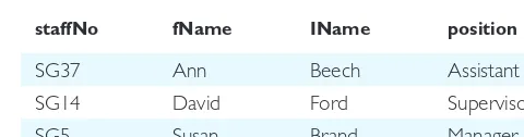
Retrieve all rows

EXAMPLE 6.1 Retrieve all columns, all rows

List full details of all staff.

Because there are no restrictions specified in this query, the WHERE clause is unneces-sary and all columns are required. We write this query as:

SELECTstaffNo, fName, IName, position, sex, DOB, salary, branchNo

FROMStaff;

Because many SQL retrievals require all columns of a table, there is a quick way of expressing “all columns” in SQL, using an asterisk (*) in place of the column names. The following statement is an equivalent and shorter way of expressing this query:

SELECT *

FROMStaff;

The result table in either case is shown in Table 6.1.

TABLE 6.1 Result table for Example 6.1.

staffNo fName IName position sex DOB salary branchNo

SL21 John White Manager M l-Oct-45 30000.00 B005

SG37 Ann Beech Assistant F l0-Nov-60 12000.00 B003

SG14 David Ford Supervisor M 24-Mar-58 18000.00 B003

SA9 Mary Howe Assistant F 19-Feb-70 9000.00 B007

SG5 Susan Brand Manager F 3-Jun-40 24000.00 B003

(10)

EXAMPLE 6.2 Retrieve specific columns, all rows

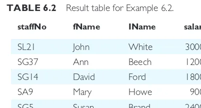
Produce a list of salaries for all staff, showing only the staff number, the first and last names, and the salary details.

SELECTstaffNo, fName, IName, salary

FROMStaff;

In this example a new table is created from Staff containing only the designated columns

staffNo, fName, IName, and salary, in the specified order. The result of this operation is shown in Table 6.2. Note that, unless specified, the rows in the result table may not be sorted. Some DBMSs do sort the result table based on one or more columns (for example, Microsoft Office Access would sort this result table based on the primary key

staffNo). We describe how to sort the rows of a result table in the next section.

staffNo fName IName salary

SL21 John White 30000.00

SG37 Ann Beech 12000.00

SG14 David Ford 18000.00

SA9 Mary Howe 9000.00

SG5 Susan Brand 24000.00

SL41 Julie Lee 9000.00

EXAMPLE 6.3 Use of DISTINCT

List the property numbers of all properties that have been viewed.

SELECTpropertyNo

FROMViewing;

The result table is shown in Table 6.3(a). Notice that there are several duplicates, because unlike the relational algebra Projection operation (see Section 5.1.1), SELECT does not

TABLE 6.3(a) Result table for

Example 6.3 with duplicates.

propertyNo

(11)

eliminate duplicates when it projects over one or more columns. To eliminate the dupli-cates, we use the DISTINCT keyword. Rewriting the query as:

SELECT DISTINCTpropertyNo

FROMViewing;

we get the result table shown in Table 6.3(b) with the duplicates eliminated.

TABLE 6.3(b) Result table for Example

6.3 with duplicates eliminated.

propertyNo

PA14 PG4 PG36

EXAMPLE 6.4 Calculated fields

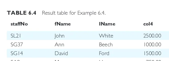
Produce a list of monthly salaries for all staff, showing the staff number, the first and last names, and the salary details.

SELECTstaffNo, fName, IName, salary/12

FROMStaff;

This query is almost identical to Example 6.2, with the exception that monthly salaries are required. In this case, the desired result can be obtained by simply dividing the salary by 12, giving the result table shown in Table 6.4.

This is an example of the use of a calculated field (sometimes called a computed or derived field). In general, to use a calculated field, you specify an SQL expression in the SELECT list. An SQL expression can involve addition, subtraction, multiplication, and division, and parentheses can be used to build complex expressions. More than one table column can be used in a calculated column; however, the columns referenced in an arithmetic expression must have a numeric type.

The fourth column of this result table has been output as col4. Normally, a column in the result table takes its name from the corresponding column of the database table from which it has been retrieved. However, in this case, SQL does not know how to label the column. Some dialects give the column a name corresponding to its position

staffNo fName IName col4

(12)

in the table (for example, col4); some may leave the column name blank or use the expression entered in the SELECT list. The ISO standard allows the column to be named using an AS clause. In the previous example, we could have written:

SELECTstaffNo,fName,IName,salary/12ASmonthlySalary

FROMStaff;

In this case, the column heading of the result table would be monthlySalary rather than col4.

Row selection (WHERE clause)

The previous examples show the use of the SELECT statement to retrieve all rows from a table. However, we often need to restrict the rows that are retrieved. This can be achieved with the WHERE clause, which consists of the keyword WHERE followed by a search condition that specifies the rows to be retrieved. The five basic search conditions (or predicates, using the ISO terminology) are as follows:

• Comparison Compare the value of one expression to the value of another expression.

• Range Test whether the value of an expression falls within a specified range of values.

• Set membership Test whether the value of an expression equals one of a set of values.

• Pattern match Test whether a string matches a specified pattern. • Null Test whether a column has a null (unknown) value.

The WHERE clause is equivalent to the relational algebra Selection operation discussed in Section 5.1.1. We now present examples of each of these types of search conditions.

EXAMPLE 6.5 Comparison search condition

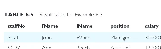
List all staff with a salary greater than £10,000.

SELECTstaffNo, fName, IName, position, salary

FROMStaff

WHEREsalary > 10000;

Here, the table is Staff and the predicate is salary > 10000. The selection creates a new table containing only those Staff rows with a salary greater than £10,000. The result of this operation is shown in Table 6.5.

staffNo fName IName position salary

SL21 John White Manager 30000.00

SG37 Ann Beech Assistant 12000.00

SG14 David Ford Supervisor 18000.00

(13)

In SQL, the following simple comparison operators are available:

= equals

<> is not equal to (ISO standard) ! = is not equal to (allowed in some dialects)

< is less than < = is less than or equal to > is greater than > = is greater than or equal to

More complex predicates can be generated using the logical operators AND, OR, and NOT, with parentheses (if needed or desired) to show the order of evaluation. The rules for evaluating a conditional expression are:

• an expression is evaluated left to right; • subexpressions in brackets are evaluated first; • NOTs are evaluated before ANDs and ORs; • ANDs are evaluated before ORs.

The use of parentheses is always recommended, in order to remove any possible ambiguities.

EXAMPLE 6.6 Compound comparison search condition

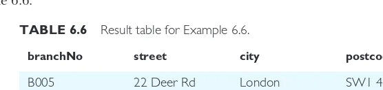
List the addresses of all branch offices in London or Glasgow.

SELECT *

FROMBranch

WHEREcity = ‘London’ ORcity = ‘Glasgow’;

In this example the logical operator OR is used in the WHERE clause to find the branches in London (city = ‘London’) or in Glasgow (city = ‘Glasgow’). The result table is shown in Table 6.6.

branchNo street city postcode

B005 22 Deer Rd London SW1 4EH

B003 163 Main St Glasgow G11 9QX

B002 56 Clover Dr London NW10 6EU

EXAMPLE 6.7 Range search condition (BETWEEN/NOT BETWEEN)

List all staff with a salary between £20,000 and £30,000.

FROMStaff

WHEREsalaryBETWEEN 20000 AND 30000;

(14)

There is also a negated version of the range test (NOT BETWEEN) that checks for values outside the range. The BETWEEN test does not add much to the expressive power of SQL, because it can be expressed equally well using two comparison tests. We could have expressed the previous query as:

FROM Staff

WHEREsalary > = 20000 ANDsalary < = 30000;

However, the BETWEEN test is a simpler way to express a search condition when con-sidering a range of values.

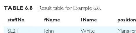
EXAMPLE 6.8 Set membership search condition (IN/NOT IN)

List all managers and supervisors.

SELECTstaffNo, fName, IName, position

FROMStaff

WHEREposition IN (‘Manager’, ‘Supervisor’);

The set membership test (IN) tests whether a data value matches one of a list of values, in this case either ‘Manager’ or ‘Supervisor’. The result table is shown in Table 6.8.

SG5 Susan Brand Manager 24000.00

staffNo fName IName position

SL21 John White Manager

SG14 David Ford Supervisor

SG5 Susan Brand Manager

There is a negated version (NOT IN) that can be used to check for data values that do not lie in a specific list of values. Like BETWEEN, the IN test does not add much to the expressive power of SQL. We could have expressed the previous query as:

FROMStaff

WHEREposition = ‘Manager’ ORposition = ‘Supervisor’;

(15)

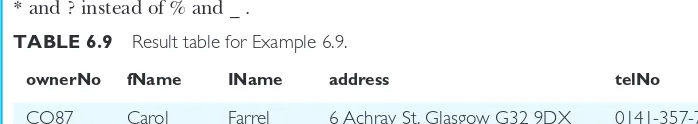
EXAMPLE 6.9 Pattern match search condition (LIKE/NOT LIKE)

Find all owners with the string ‘Glasgow’ in their address.

For this query, we must search for the string ‘Glasgow’ appearing somewhere within the

address column of the PrivateOwner table. SQL has two special pattern-matching symbols:

• The % percent character represents any sequence of zero or more characters (wildcard).

• The _ underscore character represents any single character.

All other characters in the pattern represent themselves. For example:

• address LIKE ‘H%’ means the first character must be H, but the rest of the string can be anything.

• address LIKE ‘H_ _ _’ means that there must be exactly four characters in the string, the first of which must be an H.

• address LIKE ‘%e’ means any sequence of characters, of length at least 1, with the last character an e.

• address LIKE ‘%Glasgow%’ means a sequence of characters of any length containing

Glasgow.

• address NOT LIKE ‘H%’ means the first character cannot be an H.

If the search string can include the pattern-matching character itself, we can use an escape character to represent the pattern-matching character. For example, to check for the string ‘15%’, we can use the predicate:

LIKE ‘15#%’ ESCAPE ‘#’

Using the pattern-matching search condition of SQL, we can find all owners with the string “Glasgow” in their address using the following query, producing the result table shown in Table 6.9:

SELECTownerNo, fName, IName, address, telNo

FROMPrivateOwner

WHEREaddressLIKE ‘%Glasgow%’;

Note that some RDBMSs, such as Microsoft Office Access, use the wildcard characters * and ? instead of % and _ .

ownerNo fName IName address telNo

CO87 Carol Farrel 6 Achray St, Glasgow G32 9DX 0141-357-7419

CO40 Tina Murphy 63 Well St, Glasgow G42 0141-943-1728

CO93 Tony Shaw 12 Park PI, Glasgow G4 0QR 0141-225-7025

EXAMPLE 6.10 NULL search condition (IS NULL/IS NOT NULL)

List the details of all viewings on property PG4 where a comment has not been supplied.

(16)

you may think that the latter row could be accessed by using one of the search conditions:

(propertyNo=‘PG4’ANDcomment=‘ ’)

or

(propertyNo = ‘PG4’ ANDcomment< >‘too remote’)

However, neither of these conditions would work. A null comment is considered to have an unknown value, so we cannot test whether it is equal or not equal to another string. If we tried to execute the SELECT statement using either of these compound conditions, we would get an empty result table. Instead, we have to test for null explicitly using the special keyword IS NULL:

SELECTclientNo, viewDate

FROMViewing

WHEREpropertyNo=‘PG4’ANDcommentISNULL;

The result table is shown in Table 6.10. The negated version (IS NOT NULL) can be used to test for values that are not null.

clientNo viewDate

CR56 26-May-13

6.3.2 Sorting Results (ORDER BY Clause)

In general, the rows of an SQL query result table are not arranged in any particular order (although some DBMSs may use a default ordering based, for example, on a primary key). However, we can ensure the results of a query are sorted using the ORDER BY clause in the SELECT statement. The ORDER BY clause consists of a list of column identifiers that the result is to be sorted on, separated by commas. A column identifier may be either a column name or a column number†_that

identi-fies an element of the SELECT list by its position within the list, 1 being the first (leftmost) element in the list, 2 the second element in the list, and so on. Column numbers could be used if the column to be sorted on is an expression and no AS clause is specified to assign the column a name that can subsequently be referenced. The ORDER BY clause allows the retrieved rows to be ordered in ascending (ASC) or descending (DESC) order on any column or combination of columns, regardless of whether that column appears in the result. However, some dialects insist that the ORDER BY elements appear in the SELECT list. In either case, the ORDER BY clause must always be the last clause of the SELECT statement.

(17)

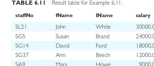
EXAMPLE 6.11 Single-column ordering

Produce a list of salaries for all staff, arranged in descending order of salary.

SELECTstaffNo, fName, IName, salary

FROMStaff

ORDER BYsalaryDESC;

This example is very similar to Example 6.2. The difference in this case is that the output is to be arranged in descending order of salary. This is achieved by adding the ORDER BY clause to the end of the SELECT statement, specifying salary as the column to be sorted, and DESC to indicate that the order is to be descending. In this case, we get the result table shown in Table 6.11. Note that we could have expressed the ORDER BY clause as: ORDER BY 4 DESC, with the 4 relating to the fourth column name in the SELECT list, namely salary.

staffNo fName IName salary

SL41 Julie Lee 9000.00

It is possible to include more than one element in the ORDER BY clause. The

major sort key determines the overall order of the result table. In Example 6.11, the major sort key is salary. If the values of the major sort key are unique, there is no need for additional keys to control the sort. However, if the values of the major sort key are not unique, there may be multiple rows in the result table with the same value for the major sort key. In this case, it may be desirable to order rows with the same value for the major sort key by some additional sort key. If a second element appears in the ORDER BY clause, it is called a minor sort key.

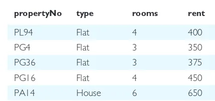
EXAMPLE 6.12 Multiple column ordering

Produce an abbreviated list of properties arranged in order of property type.

SELECTpropertyNo, type, rooms, rent

FROMPropertyForRent

ORDER BYtype;

In this case we get the result table shown in Table 6.12(a).

(18)

SELECTpropertyNo, type, rooms, rent

ORDER BYtype, rentDESC;

TABLE 6.12(a) Result table for Example 6.12 with one sort key.

propertyNo type rooms rent

PL94 Flat 4 400

PG4 Flat 3 350

PG36 Flat 3 375

PG16 Flat 4 450

PA14 House 6 650

PG21 House 5 600

Now, the result is ordered first by property type, in ascending alphabetic order (ASC being the default setting), and within property type, in descending order of rent. In this case, we get the result table shown in Table 6.12(b).

TABLE 6.12(b) Result table for Example 6.12 with two sort keys.

propertyNo type rooms rent

PG16 Flat 4 450

PL94 Flat 4 400

PG36 Flat 3 375

PG4 Flat 3 350

PA14 House 6 650

PG21 House 5 600

The ISO standard specifies that nulls in a column or expression sorted with ORDER BY should be treated as either less than all nonnull values or greater than all nonnull values. The choice is left to the DBMS implementor.

6.3.3 Using the SQL Aggregate Functions

As well as retrieving rows and columns from the database, we often want to per-form some per-form of summation or aggregation of data, similar to the totals at the bottom of a report. The ISO standard defines five aggregate functions:

(19)

These functions operate on a single column of a table and return a single value. COUNT, MIN, and MAX apply to both numeric and nonnumeric fields, but SUM and AVG may be used on numeric fields only. Apart from COUNT(*), each func-tion eliminates nulls first and operates only on the remaining nonnull values. COUNT(*) is a special use of COUNT that counts all the rows of a table, regardless of whether nulls or duplicate values occur.

If we want to eliminate duplicates before the function is applied, we use the key-word DISTINCT before the column name in the function. The ISO standard allows the keyword ALL to be specified if we do not want to eliminate duplicates, although ALL is assumed if nothing is specified. DISTINCT has no effect with the MIN and MAX functions. However, it may have an effect on the result of SUM or AVG, so consideration must be given to whether duplicates should be included or excluded in the computation. In addition, DISTINCT can be specified only once in a query.

It is important to note that an aggregate function can be used only in the SELECT list and in the HAVING clause (see Section 6.3.4). It is incorrect to use it elsewhere. If the SELECT list includes an aggregate function and no GROUP BY clause is being used to group data together (see Section 6.3.4), then no item in the SELECT list can include any reference to a column unless that column is the argu-ment to an aggregate function. For example, the following query is illegal:

SELECTstaffNo,COUNT(salary)

FROMStaff;

because the query does not have a GROUP BY clause and the column staffNo in the SELECT list is used outside an aggregate function.

EXAMPLE 6.13 Use of COUNT(*)

How many properties cost more than £350 per month to rent?

SELECT COUNT(*) ASmyCount

WHERErent> 350;

Restricting the query to properties that cost more than £350 per month is achieved using the WHERE clause. The total number of properties satisfying this condition can then be found by applying the aggregate function COUNT. The result table is shown in Table 6.13.

EXAMPLE 6.14 Use of COUNT(DISTINCT)

How many different properties were viewed in May 2013?

SELECT COUNT(DISTINCTpropertyNo) ASmyCount

FROMViewing

WHEREviewDateBETWEEN ‘1-May-13’ AND ‘31-May-13’;

Again, restricting the query to viewings that occurred in May 2013 is achieved using the WHERE clause. The total number of viewings satisfying this condition can then be found by applying the aggregate function COUNT. However, as the same property may be viewed many times, we have to use the DISTINCT keyword to eliminate duplicate properties. The result table is shown in Table 6.14.

(20)

EXAMPLE 6.15 Use of COUNT and SUM

Find the total number of Managers and the sum of their salaries.

SELECT COUNT(staffNo)ASmyCount,SUM(salary)ASmySum

FROMStaff

WHEREposition = ‘Manager’;

Restricting the query to Managers is achieved using the WHERE clause. The number of Managers and the sum of their salaries can be found by applying the COUNT and the SUM functions respectively to this restricted set. The result table is shown in Table 6.15.

TABLE 6.15 Result table for

Example 6.15.

myCount mySum

2 54000.00

EXAMPLE 6.16 Use of MlN, MAX, AVG

Find the minimum, maximum, and average staff salary.

SELECTMIN(salary)ASmyMin,MAX(salary)ASmyMax,AVG(salary)ASmyAvg

FROMStaff;

In this example, we wish to consider all staff and therefore do not require a WHERE clause. The required values can be calculated using the MIN, MAX, and AVG functions based on the salary column. The result table is shown in Table 6.16.

myMin myMax myAvg

9000.00 30000.00 17000.00

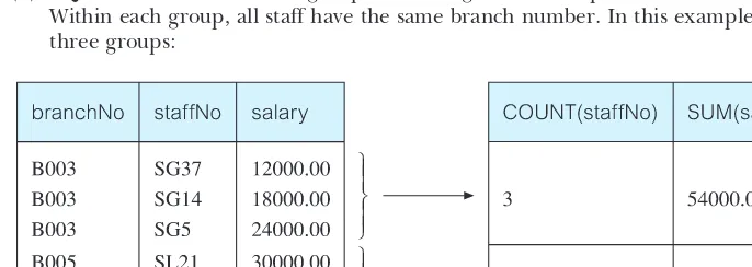
6.3.4 Grouping Results (GROUP BY Clause)

The previous summary queries are similar to the totals at the bottom of a report. They condense all the detailed data in the report into a single summary row of data. However, it is often useful to have subtotals in reports. We can use the GROUP BY clause of the SELECT statement to do this. A query that includes the GROUP BY clause is called a grouped query, because it groups the data from the SELECT table(s) and produces a single summary row for each group. The columns named in the GROUP BY clause are called the grouping columns. The ISO standard requires the SELECT clause and the GROUP BY clause to be closely integrated. When GROUP BY is used, each item in the SELECT list must be single-valued per group. In addition, the SELECT clause may contain only:

(21)

• constants;

• an expression involving combinations of these elements.

All column names in the SELECT list must appear in the GROUP BY clause unless the name is used only in an aggregate function. The contrary is not true: there may be column names in the GROUP BY clause that do not appear in the SELECT list. When the WHERE clause is used with GROUP BY, the WHERE clause is applied first, then groups are formed from the remaining rows that satisfy the search condition.

The ISO standard considers two nulls to be equal for purposes of the GROUP BY clause. If two rows have nulls in the same grouping columns and identical values in all the nonnull grouping columns, they are combined into the same group.

EXAMPLE 6.17 Use of GROUP BY

Find the number of staff working in each branch and the sum of their salaries.

SELECTbranchNo,COUNT(staffNo)ASmyCount,SUM(salary)ASmySum

FROMStaff

GROUP BYbranchNo

ORDER BYbranchNo;

It is not necessary to include the column names staffNo and salary in the GROUP BY list, because they appear only in the SELECT list within aggregate functions. On the other hand, branchNo is not associated with an aggregate function and so must appear in the GROUP BY list. The result table is shown in Table 6.17.

branchNo myCount mySum

B003 3 54000.00

B005 2 39000.00

B007 1 9000.00

Conceptually, SQL performs the query as follows:

(22)

(2) For each group, SQL computes the number of staff members and calculates the sum of the values in the salary column to get the total of their salaries. SQL generates a single summary row in the query result for each group.

(3) Finally, the result is sorted in ascending order of branch number, branchNo. The SQL standard allows the SELECT list to contain nested queries (see Section 6.3.5). Therefore, we could also express the previous query as:

SELECTbranchNo,(SELECTCOUNT(staffNo)ASmyCount

FROMStaff s

WHEREs.branchNo = b.branchNo),

(SELECT SUM(salary)ASmySum

FROMStaff s

WHEREs.branchNo = b.branchNo)

FROMBranch b

With this version of the query, however, the two aggregate values are produced for each branch office in Branch; in some cases possibly with zero values.

Restricting groupings (HAVING clause)

The HAVING clause is designed for use with the GROUP BY clause to restrict the

groups that appear in the final result table. Although similar in syntax, HAVING and WHERE serve different purposes. The WHERE clause filters individual rows going into the final result table, whereas HAVING filters groups going into the final result table. The ISO standard requires that column names used in the HAVING clause must also appear in the GROUP BY list or be contained within an aggregate function. In practice, the search condition in the HAVING clause always includes at least one aggregate function; otherwise the search condition could be moved to the WHERE clause and applied to individual rows. (Remember that aggregate functions cannot be used in the WHERE clause.)

The HAVING clause is not a necessary part of SQL—any query expressed using a HAVING clause can always be rewritten without the HAVING clause.

EXAMPLE 6.18 Use of HAVING

For each branch office with more than one member of staff, find the number of staff working in each branch and the sum of their salaries.

SELECTbranchNo,COUNT(staffNo)ASmyCount,SUM(salary)ASmySum

FROMStaff

GROUP BYbranchNo

HAVING COUNT(staffNo) > 1

(23)

6.3.5 Subqueries

In this section we examine the use of a complete SELECT statement embedded within another SELECT statement. The results of this inner SELECT statement (or subselect) are used in the outer statement to help determine the contents of the final result. A sub-select can be used in the WHERE and HAVING clauses of an outer SELECT statement, where it is called a subquery or nested query. Subselects may also appear in INSERT, UPDATE, and DELETE statements (see Section 6.3.10). There are three types of subquery:

• A scalar subquery returns a single column and a single row, that is, a single value. In principle, a scalar subquery can be used whenever a single value is needed. Example 6.19 uses a scalar subquery.

• A row subquery returns multiple columns, but only a single row. A row subquery can be used whenever a row value constructor is needed, typically in predicates. • A table subquery returns one or more columns and multiple rows. A table

sub-query can be used whenever a table is needed, for example, as an operand for the IN predicate.

EXAMPLE 6.19 Using a subquery with equality

List the staff who work in the branch at ‘163 Main St’.

FROMStaff

WHEREbranchNo = (SELECTbranchNo

FROMBranch

WHEREstreet = ‘163 Main St’);

The inner SELECT statement (SELECT branchNo FROM Branch . . .) finds the branch number that corresponds to the branch with street name ‘163 Main St’ (there will be only one such branch number, so this is an example of a scalar subquery). Having obtained this branch number, the outer SELECT statement then retrieves the details of all staff who work at this branch. In other words, the inner SELECT returns a result table containing a single value ‘B003’, corresponding to the branch at ‘163 Main St’, and the outer SELECT becomes:

FROMStaff

WHEREbranchNo = ‘B003’;

The result table is shown in Table 6.19.

branchNo myCount mySum

B003 3 54000.00

(24)

We can think of the subquery as producing a temporary table with results that can be accessed and used by the outer statement. A subquery can be used immediately following a relational operator (=, <, >, <=, > =,< >) in a WHERE clause, or a HAVING clause. The subquery itself is always enclosed in parentheses.

EXAMPLE 6.20 Using a subquery with an aggregate function

List all staff whose salary is greater than the average salary, and show by how much their salary is greater than the average.

SELECTstaffNo, fName, IName, position,

salary – (SELECT AVG(salary)FROMStaff)ASsalDiff

FROMStaff

WHEREsalary > (SELECT AVG(salary)FROMStaff);

First, note that we cannot write ‘WHERE salary > AVG(salary)’, because aggregate func-tions cannot be used in the WHERE clause. Instead, we use a subquery to find the aver-age salary, and then use the outer SELECT statement to find those staff with a salary greater than this average. In other words, the subquery returns the average salary as £17,000. Note also the use of the scalar subquery in the SELECT list to determine the difference from the average salary. The outer query is reduced then to:

SELECTstaffNo, fName, IName, position, salary – 17000ASsalDiff

FROMStaff

WHEREsalary> 17000;

The result table is shown in Table 6.20.

SG37 Ann Beech Assistant

SG14 David Ford Supervisor

SG5 Susan Brand Manager

staffNo fName IName position salDiff

The following rules apply to subqueries:

(25)

(2) The subquery SELECT list must consist of a single column name or expression, except for subqueries that use the keyword EXISTS (see Section 6.3.8).

(3) By default, column names in a subquery refer to the table name in the FROM clause of the subquery. It is possible to refer to a table in a FROM clause of an outer query by qualifying the column name (see following).

(4) When a subquery is one of the two operands involved in a comparison, the subquery must appear on the right-hand side of the comparison. For example, it would be incorrect to express the previous example as:

FROMStaff

WHERE (SELECT AVG(salary)FROMStaff) < salary;

because the subquery appears on the left-hand side of the comparison with salary.

EXAMPLE 6.21 Nested subqueries: use of IN

List the properties that are handled by staff who work in the branch at ‘163 Main St’.

SELECTpropertyNo, street, city, postcode, type, rooms, rent

WHEREstaffNoIN(SELECTstaffNo

FROMStaff

WHEREbranchNo=(SELECTbranchNo

FROMBranch

WHEREstreet= ‘163 Main St’)); Working from the innermost query outwards, the first query selects the number of the branch at ‘163 Main St’. The second query then selects those staff who work at this branch number. In this case, there may be more than one such row found, and so we cannot use the equality condition (=) in the outermost query. Instead, we use the IN keyword. The outermost query then retrieves the details of the properties that are managed by each member of staff identified in the middle query. The result table is shown in Table 6.21.

propertyNo street city postcode type rooms rent

PG16 5 Novar Dr Glasgow G12 9AX Flat 4 450

PG36 2 Manor Rd Glasgow G32 4QX Flat 3 375

PG21 18 Dale Rd Glasgow G12 House 5 600

6.3.6 ANY and ALL

(26)

empty, the ALL condition returns true, the ANY condition returns false. The ISO standard also allows the qualifier SOME to be used in place of ANY.

EXAMPLE 6.22 Use of ANY/SOME

Find all staff whose salary is larger than the salary of at least one member of staff at branch B003.

FROMStaff

WHEREsalary > SOME(SELECTsalary

FROMStaff

WHEREbranchNo= ‘B003’);

Although this query can be expressed using a subquery that finds the minimum salary of the staff at branch B003 and then an outer query that finds all staff whose salary is greater than this number (see Example 6.20), an alternative approach uses the SOME/ ANY keyword. The inner query produces the set {12000, 18000, 24000} and the outer query selects those staff whose salaries are greater than any of the values in this set (that is, greater than the minimum value, 12000). This alternative method may seem more natural than finding the minimum salary in a subquery. In either case, the result table is shown in Table 6.22.

EXAMPLE 6.23 Use of ALL

Find all staff whose salary is larger than the salary of every member of staff at branch B003.

FROMStaff

WHEREsalary > ALL(SELECTsalary

FROMStaff

WHEREbranchNo= ‘B003’);

This example is very similar to the previous example. Again, we could use a subquery to find the maximum salary of staff at branch B003 and then use an outer query to find all staff whose salary is greater than this number. However, in this example we use the ALL keyword. The result table is shown in Table 6.23.

(27)

6.3.7 Multi-table Queries

All the examples we have considered so far have a major limitation: the columns that are to appear in the result table must all come from a single table. In many cases, this is insufficient to answer common queries that users will have. To combine columns from several tables into a result table, we need to use a join operation. The SQL join operation combines information from two tables by forming pairs of related rows from the two tables. The row pairs that make up the joined table are those where the matching columns in each of the two tables have the same value.

If we need to obtain information from more than one table, the choice is between using a subquery and using a join. If the final result table is to contain columns from different tables, then we must use a join. To perform a join, we simply include more than one table name in the FROM clause, using a comma as a separator, and typically including a WHERE clause to specify the join column(s). It is also possible to use an alias for a table named in the FROM clause. In this case, the alias is sepa-rated from the table name with a space. An alias can be used to qualify a column name whenever there is ambiguity regarding the source of the column name. It can also be used as a shorthand notation for the table name. If an alias is provided, it can be used anywhere in place of the table name.

EXAMPLE 6.24 Simple join

List the names of all clients who have viewed a property, along with any comments supplied.

SELECTc.clientNo, fName, IName, propertyNo, comment

FROMClient c, Viewing v

WHEREc.clientNo = v.clientNo;

We want to display the details from both the Client table and the Viewing table, and so we have to use a join. The SELECT clause lists the columns to be displayed. Note that it is necessary to qualify the client number, clientNo, in the SELECT list: clientNo could come from either table, and we have to indicate which one. (We could also have chosen the clientNo column from the Viewing table.) The qualification is achieved by prefixing the column name with the appropriate table name (or its alias). In this case, we have used c as the alias for the Client table.

To obtain the required rows, we include those rows from both tables that have identi-cal values in the clientNo columns, using the search condition (c.clientNo = v.clientNo). We call these two columns the matching columns for the two tables. This is equivalent to the relational algebra Equijoin operation discussed in Section 5.1.3. The result table is shown in Table 6.24.

clientNo fName IName propertyNo comment

CR56 Aline Stewart PG36

CR56 Aline Stewart PA14 too small

CR56 Aline Stewart PG4

CR62 Mary Tregear PA14 no dining room

(28)

The most common multi-table queries involve two tables that have a one-to-many (1:*) (or a parent/child) relationship (see Section 12.6.2). The previous query involving clients and viewings is an example of such a query. Each viewing (child) has an associated client (parent), and each client (parent) can have many associated viewings (children). The pairs of rows that generate the query results are parent/ child row combinations. In Section 4.2.5 we described how primary key and foreign keys create the parent/child relationship in a relational database: the table contain-ing the primary key is the parent table and the table containcontain-ing the foreign key is the child table. To use the parent/child relationship in an SQL query, we specify a search condition that compares the primary key and the foreign key. In Example 6.24, we compared the primary key in the Client table, c.clientNo, with the foreign key in the Viewing table, v.clientNo.

The SQL standard provides the following alternative ways to specify this join:

FROMClient cJOINViewing vONc.clientNo = v.clientNo

FROMClientJOINViewingUSINGclientNo

FROMClientNATURAL JOINViewing

In each case, the FROM clause replaces the original FROM and WHERE clauses. However, the first alternative produces a table with two identical clientNo columns; the remaining two produce a table with a single clientNo column.

EXAMPLE 6.25 Sorting a join

For each branch office, list the staff numbers and names of staff who manage properties and the properties that they manage.

SELECTs.branchNo, s.staffNo, fName, IName, propertyNo

FROMStaff s, PropertyForRent p

WHEREs.staffNo = p.staffNo

ORDER BYs.branchNo, s.staffNo, propertyNo;

In this example, we need to join the Staff and PropertyForRent tables, based on the primary key/foreign key attribute (staffNo). To make the results more readable, we have ordered the output using the branch number as the major sort key and the staff number and property number as the minor keys. The result table is shown in Table 6.25.

branchNo staffNo fName IName propertyNo

B003 SG14 David Ford PG16

B003 SG37 Ann Beech PG21

B003 SG37 Ann Beech PG36

B005 SL41 Julie Lee PL94

(29)

EXAMPLE 6.26 Three-table join

For each branch, list the staff numbers and names of staff who manage properties, including the city in which the branch is located and the properties that the staff manage.

SELECTb.branchNo, b.city, s.staffNo, fName, IName, propertyNo

FROMBranch b, Staff s, PropertyForRent p

WHEREb.branchNo = s.branchNoANDs.staffNo = p.staffNo

ORDER BYb.branchNo, s.staffNo, propertyNo;

The result table requires columns from three tables: Branch (branchNo and city), Staff

(staffNo, fName and lName), and PropertyForRent (propertyNo), so a join must be used. The

Branch and Staff details are joined using the condition (b.branchNo = s.branchNo) to link each branch to the staff who work there. The Staff and PropertyForRent details are joined using the condition (s.staffNo = p.staffNo) to link staff to the properties they manage. The result table is shown in Table 6.26.

branchNo city staffNo fName IName propertyNo

B003 Glasgow SG14 David Ford PG16

B003 Glasgow SG37 Ann Beech PG21

B003 Glasgow SG37 Ann Beech PG36

B005 London SL41 Julie Lee PL94

B007 Aberdeen SA9 Mary Howe PA14

Note again that the SQL standard provides alternative formulations for the FROM and WHERE clauses, for example:

FROM (Branch bJOINStaff sUSINGbranchNo) ASbs

JOINPropertyForRentpUSINGstaffNo

EXAMPLE 6.27 Multiple grouping columns

Find the number of properties handled by each staff member, along with the branch number of the member of staff.

SELECTs.branchNo, s.staffNo,COUNT(*) ASmyCount

FROMStaff s, PropertyForRent p

WHEREs.staffNo = p.staffNo

GROUP BYs.branchNo, s.staffNo

ORDER BYs.branchNo, s.staffNo;

To list the required numbers, we first need to find out which staff actually manage properties. This can be found by joining the Staff and PropertyForRent tables on the

(30)

Computing a join

A join is a subset of a more general combination of two tables known as the

Cartesian product (see Section 5.1.2). The Cartesian product of two tables is another table consisting of all possible pairs of rows from the two tables. The columns of the product table are all the columns of the first table followed by all the columns of the second table. If we specify a two-table query without a WHERE clause, SQL produces the Cartesian product of the two tables as the query result. In fact, the ISO standard provides a special form of the SELECT statement for the Cartesian product:

SELECT [DISTINCT | ALL] {* | columnList}

FROM TableName1CROSS JOINTableName2

Consider again Example 6.24, where we joined the Client and Viewing tables using the matching column, clientNo. Using the data from Figure 4.3, the Cartesian prod-uct of these two tables would contain 20 rows (4 clients * 5 viewings = 20 rows). It is equivalent to the query used in Example 6.24 without the WHERE clause.

Conceptually, the procedure for generating the results of a SELECT with a join is as follows:

(1) Form the Cartesian product of the tables named in the FROM clause.

(2) If there is a WHERE clause, apply the search condition to each row of the product table, retaining those rows that satisfy the condition. In terms of the relational algebra, this operation yields a restriction of the Cartesian product. (3) For each remaining row, determine the value of each item in the SELECT list

to produce a single row in the result table.

(4) If SELECT DISTINCT has been specified, eliminate any duplicate rows from the result table. In the relational algebra, Steps 3 and 4 are equivalent to a

projection of the restriction over the columns mentioned in the SELECT list. (5) If there is an ORDER BY clause, sort the result table as required.

We will discuss query processing in more detail in Chapter 23.

Outer joins

The join operation combines data from two tables by forming pairs of related rows where the matching columns in each table have the same value. If one row of a

TABLE 6.27(a) Result table for Example 6.27.

branchNo staffNo myCount

B003 SG14 1

B003 SG37 2

B005 SL41 1

(31)

table is unmatched, the row is omitted from the result table. This has been the case for the joins we examined earlier. The ISO standard provides another set of join operators called outer joins (see Section 5.1.3). The Outer join retains rows that do not satisfy the join condition. To understand the Outer join operators, consider the following two simplified Branch and PropertyForRent tables, which we refer to as

Branch1 and PropertyForRent1, respectively:

Branch1

branchNo bCity

B003 Glasgow

B004 Bristol

B002 London

PropertyForRent1

propertyNo pCity

PA14 Aberdeen

PL94 London

PG4 Glasgow

The (Inner) join of these two tables:

SELECTb.*, p.*

FROMBranch1 b, PropertyForRent1 p

WHEREb.bCity = p.pCity;

produces the result table shown in Table 6.27(b).

TABLE 6.27(b) Result table for inner join of the Branch1

and PropertyForRent1 tables.

branchNo bCity propertyNo pCity

B003 Glasgow PG4 Glasgow

B002 London PL94 London

The result table has two rows where the cities are the same. In particular, note that there is no row corresponding to the branch office in Bristol and there is no row corresponding to the property in Aberdeen. If we want to include the unmatched rows in the result table, we can use an Outer join. There are three types of Outer join: Left, Right, and Full Outer joins. We illustrate their functionality in the following examples.

EXAMPLE 6.28 Left Outer join

List all branch offices and any properties that are in the same city.

The Left Outer join of these two tables:

SELECTb.*, p.*

(32)

produces the result table shown in Table 6.28. In this example the Left Outer join includes not only those rows that have the same city, but also those rows of the first (left) table that are unmatched with rows from the second (right) table. The columns from the second table are filled with NULLs.

B004 Bristol NULL NULL

EXAMPLE 6.29 Right Outer join

List all properties and any branch offices that are in the same city.

The Right Outer join of these two tables:

SELECTb.*, p.*

FROMBranch1 bRIGHT JOINPropertyForRent1 pONb.bCity = p.pCity;

produces the result table shown in Table 6.29. In this example, the Right Outer join includes not only those rows that have the same city, but also those rows of the second (right) table that are unmatched with rows from the first (left) table. The columns from the first table are filled with NULLs.

NULL NULL PA14 Aberdeen

EXAMPLE 6.30 Full Outer join

List the branch offices and properties that are in the same city along with any unmatched branches or properties.

The Full Outer join of these two tables:

SELECTb.*, p.*

(33)

produces the result table shown in Table 6.30. In this case, the Full Outer join includes not only those rows that have the same city, but also those rows that are unmatched in both tables. The unmatched columns are filled with NULLs.

NULL NULL PA14 Aberdeen

B004 Bristol NULL NULL

6.3.8 EXISTS and NOT EXISTS

The keywords EXISTS and NOT EXISTS are designed for use only with subquer-ies. They produce a simple true/false result. EXISTS is true if and only if there exists at least one row in the result table returned by the subquery; it is false if the subquery returns an empty result table. NOT EXISTS is the opposite of EXISTS. Because EXISTS and NOT EXISTS check only for the existence or nonexistence of rows in the subquery result table, the subquery can contain any number of columns. For simplicity, it is common for subqueries following one of these keywords to be of the form:

(SELECT * FROM . . .)

EXAMPLE 6.31 Query using EXISTS

Find all staff who work in a London branch office.

FROMStaff s

WHERE EXISTS (SELECT *

FROMBranch b

WHEREs.branchNo = b.branchNo ANDcity = ‘London’);

This query could be rephrased as ‘Find all staff such that there exists a Branch row con-taining his/her branch number, branchNo, and the branch city equal to London’. The test for inclusion is the existence of such a row. If it exists, the subquery evaluates to true. The result table is shown in Table 6.31.

SL21 John White Manager