Java 9 Data Structures and Algorithms A step by step guide to data structures and algorithms pdf pdf

(1)

(2)

Java 9 Data Structures and

Algorithms

A step-by-step guide to data structures and algorithms

Debasish Ray Chawdhuri

(3)

Java 9 Data Structures and Algorithms

All rights reserved. No part of this book may be reproduced, stored in a retrieval system, or transmitted in any form or by any means, without the prior written permission of the publisher, except in the case of brief quotations embedded in critical articles or reviews.

Every effort has been made in the preparation of this book to ensure the accuracy of the information presented. However, the information contained in this book is sold without warranty, either express or implied. Neither the author, nor Packt Publishing, and its dealers and distributors will be held liable for any damages caused or alleged to be caused directly or indirectly by this book.

Packt Publishing has endeavored to provide trademark information about all of the companies and products mentioned in this book by the appropriate use of capitals. However, Packt Publishing cannot guarantee the accuracy of this information.

First published: April 2017

Production reference: 1250417

Published by Packt Publishing Ltd. Livery Place

35 Livery Street

Birmingham B3 2PB, UK.

ISBN 978-1-78588-934-9

(4)

Credits

Author

Debasish Ray Chawdhuri

Reviewer

Miroslav Wengner

Commissioning Editor Kunal Parikh

Acquisition Editor Chaitanya Nair

Content Development Editor Nikhil Borkar

Technical Editor

Madhunikita Sunil Chindarkar

Copy Editor

Muktikant Garimella

Project Coordinator Vaidehi Sawant

Proofreader

Safis Editing

Indexer

Mariammal Chettiyar

Graphics Abhinash Sahu

Production Coordinator Nilesh Mohite

(5)

About the Author

Debasish Ray Chawdhuri

is an established Java developer and has been in the industry for the last 8 years. He has developed several systems, right from CRUD applications to programming languages and big data processing systems. He had provided the first implementation of extensible business reporting language specification, and a product around it, for the verification of company financial data for the Government of India while he was employed at Tata Consultancy Services Ltd. In Talentica Software Pvt. Ltd., he implemented a domain-specific programming language to easily implement complex data aggregation computation that would compile to Java bytecode. Currently, he is leading a team developing a new high-performance structured data storage framework to be processed by Spark. The framework is named Hungry Hippos and will be open sourced very soon. He also blogs at http://www.geekyarticles.com/ about Java and other computer science-related topics.

He has worked for Tata Consultancy Services Ltd., Oracle India Pvt. Ltd., and Talentica Software Pvt. Ltd.

I would like to thank my dear wife, Anasua, for her continued support and encouragement, and for putting up with all my

(6)

About the Reviewer

Miroslav Wengner

has been a passionate JVM enthusiast ever since he joined SUN Microsystems in 2002. He truly believes in distributed system design, concurrency, and parallel computing. One of Miro's biggest hobby is the development of autonomic systems. He is one of the coauthors of and main contributors to the open source Java IoT/Robotics framework Robo4J.

Miro is currently working on the online energy trading platform for enmacc.de as a senior software developer.

(7)

www.PacktPub.com

eBooks, discount offers, and more

Did you know that Packt offers eBook versions of every book published, with PDF and ePub files available? You can upgrade to the eBook version at www.PacktPub. com and as a print book customer, you are entitled to a discount on the eBook copy. Get in touch with us at customercare@packtpub.com for more details.

At www.PacktPub.com, you can also read a collection of free technical articles, sign up for a range of free newsletters and receive exclusive discounts and offers on Packt books and eBooks.

https://www.packtpub.com/mapt

Get the most in-demand software skills with Mapt. Mapt gives you full access to all Packt books and video courses, as well as industry-leading tools to help you plan your personal development and advance your career.

Why subscribe?

• Fully searchable across every book published by Packt • Copy and paste, print, and bookmark content

(8)

Customer Feedback

Thanks for purchasing this Packt book. At Packt, quality is at the heart of our

editorial process. To help us improve, please leave us an honest review on this book's Amazon page at https://www.amazon.com/dp/1785889346.

(9)

(10)

Preface

Java has been one of the most popular programming languages for enterprise

systems for decades now. One of the reasons for the popularity of Java is its platform independence, which lets one write and compile code on any system and run it on any other system, irrespective of the hardware and the operating system. Another reason for Java's popularity is that the language is standardized by a community of industry players. The latter enables Java to stay updated with the most recent programming ideas without being overloaded with too many useless features.

Given the popularity of Java, there are plenty of developers actively involved in Java development. When it comes to learning algorithms, it is best to use the language that one is most comfortable with. This means that it makes a lot of sense to write an algorithm book, with the implementations written in Java. This book covers the most commonly used data structures and algorithms. It is meant for people who already know Java but are not familiar with algorithms. The book should serve as the first stepping stone towards learning the subject.

What this book covers

Chapter 1, Why Bother? – Basic, introduces the point of studying algorithms and data structures with examples. In doing so, it introduces you to the concept of asymptotic complexity, big O notation, and other notations.

Chapter 2, Cogs and Pulleys – Building Blocks, introduces you to array and the different kinds of linked lists, and their advantages and disadvantages. These data structures will be used in later chapters for implementing abstract data structures.

(17)

Chapter 4, Detour – Functional Programming, introduces you to the functional

programming ideas appropriate for a Java programmer. The chapter also introduces the lambda feature of Java, available from Java 8, and helps readers get used to the functional way of implementing algorithms. This chapter also introduces you to the concept of monads.

Chapter 5, Efficient Searching – Binary Search and Sorting, introduces efficient searching using binary searches on a sorted list. It then goes on to describe basic algorithms used to obtain a sorted array so that binary searching can be done.

Chapter 6, Efficient Sorting – Quicksort and Mergesort, introduces the two most popular and efficient sorting algorithms. The chapter also provides an analysis of why this is as optimal as a comparison-based sorting algorithm can ever be.

Chapter 7, Concepts of Tree, introduces the concept of a tree. It especially introduces binary trees, and also covers different traversals of the tree: breadth-first and depth-first, and pre-order, post-order, and in-order traversal of binary tree. Chapter 8, More About Search – Search Trees and Hash Tables, covers search using balanced binary search trees, namely AVL, and red-black trees and hash-tables.

Chapter 9, Advanced General Purpose Data Structures, introduces priority queues and their implementation with a heap and a binomial forest. At the end, the chapter introduces sorting with a priority queue.

Chapter 10, Concepts of Graph, introduces the concepts of directed and undirected graphs. Then, it discusses the representation of a graph in memory. Depth-first and breadth-first traversals are covered, the concept of a minimum-spanning tree is introduced, and cycle detection is discussed.

Chapter 11, Reactive Programming, introduces the reader to the concept of reactive programming in Java. This includes the implementation of an observable pattern-based reactive programming framework and a functional API on top of it. Examples are shown to demonstrate the performance gain and ease of use of the reactive framework, compared with a traditional imperative style.

What you need for this book

(18)

Who this book is for

This book is for Java developers who want to learn about data structures and algorithms. A basic knowledge of Java is assumed.

Conventions

In this book, you will find a number of text styles that distinguish between different kinds of information. Here are some examples of these styles and an explanation of their meaning.

Code words in text, database table names, folder names, filenames, file extensions, pathnames, dummy URLs, user input, and Twitter handles are shown as follows: "We can include other contexts through the use of the include directive."

A block of code is set as follows:

public static void printAllElements(int[] anIntArray){ for(int i=0;i<anIntArray.length;i++){

System.out.println(anIntArray[i]); }

}

When we wish to draw your attention to a particular part of a code block, the relevant lines or items are set in bold:

System.out.println(anIntArray[i]);

} }

Any command-line input or output is written as follows:

# cp /usr/src/asterisk-addons/configs/cdr_mysql.conf.sample /etc/asterisk/cdr_mysql.conf

(19)

Warnings or important notes appear in a box like this.

Tips and tricks appear like this.

Reader feedback

Feedback from our readers is always welcome. Let us know what you think about this book—what you liked or disliked. Reader feedback is important for us as it helps us develop titles that you will really get the most out of.

To send us general feedback, simply e-mail feedback@packtpub.com, and mention the book's title in the subject of your message.

If there is a topic that you have expertise in and you are interested in either writing or contributing to a book, see our author guide at www.packtpub.com/authors.

Customer support

Now that you are the proud owner of a Packt book, we have a number of things to help you to get the most from your purchase.

Downloading the example code

You can download the example code files for this book from your account at http:// www.packtpub.com. If you purchased this book elsewhere, you can visit http://www. packtpub.com/support and register to have the files e-mailed directly to you.

You can download the code files by following these steps:

1. Log in or register to our website using your e-mail address and password. 2. Hover the mouse pointer on the SUPPORT tab at the top.

3. Click on Code Downloads & Errata.

4. Enter the name of the book in the Search box.

(20)

You can also download the code files by clicking on the Code Files button on the book's webpage at the Packt Publishing website. This page can be accessed by

entering the book's name in the Search box. Please note that you need to be logged in to your Packt account.

Once the file is downloaded, please make sure that you unzip or extract the folder using the latest version of:

• WinRAR / 7-Zip for Windows • Zipeg / iZip / UnRarX for Mac • 7-Zip / PeaZip for Linux

The code bundle for the book is also hosted on GitHub at https://github.com/ PacktPublishing/Java-9-Data-Structures-and-Algorithms. We also have other code bundles from our rich catalog of books and videos available at https://github. com/PacktPublishing/Java9DataStructuresandAlgorithm. Check them out!

Downloading the color images of this book

We also provide you with a PDF file that has color images of the screenshots/ diagrams used in this book. The color images will help you better understand the changes in the output. You can download this file from http://www.packtpub. com/sites/default/fles/downloads/Java9DataStructuresandAlgorithms_ ColorImages.pdf.

Errata

Although we have taken every care to ensure the accuracy of our content, mistakes do happen. If you find a mistake in one of our books—maybe a mistake in the text or the code—we would be grateful if you could report this to us. By doing so, you can save other readers from frustration and help us improve subsequent versions of this book. If you find any errata, please report them by visiting http://www.packtpub. com/submit-errata, selecting your book, clicking on the Errata Submission Form link, and entering the details of your errata. Once your errata are verified, your submission will be accepted and the errata will be uploaded to our website or added to any list of existing errata under the Errata section of that title.

(21)

Piracy

Piracy of copyrighted material on the Internet is an ongoing problem across all media. At Packt, we take the protection of our copyright and licenses very seriously. If you come across any illegal copies of our works in any form on the Internet, please provide us with the location address or website name immediately so that we can pursue a remedy.

Please contact us at copyright@packtpub.com with a link to the suspected pirated material.

We appreciate your help in protecting our authors and our ability to bring you valuable content.

Questions

(22)

Why Bother? – Basic

Since you already know Java, you have of course written a few programs, which means you have written algorithms. "Well then, what is it?" you might ask. An algorithm is a list of well-defined steps that can be followed by a processor mechanically, or without involving any sort of intelligence, which would produce a desired output in a finite amount of time. Well, that's a long sentence. In simpler words, an algorithm is just an unambiguous list of steps to get something done. It kind of sounds like we are talking about a program. Isn't a program also a list of instructions that we give the computer to follow, in order to get a desired result? Yes it is, and that means an algorithm is really just a program. Well not really, but almost. An algorithm is a program without the details of the particular programming language that we are coding it in. It is the basic idea of the program; think of it as an abstraction of a program where you don't need to bother about the program's syntactic details.

Well, since we already know about programming, and an algorithm is just a program, we are done with it, right? Not really. There is a lot to learn about

programs and algorithms, that is, how to write an algorithm to achieve a particular goal. There are, of course, in general, many ways to solve a particular problem and not all ways may be equal. One way may be faster than another, and that is a very important thing about algorithms. When we study algorithms, the time it takes to execute is of utmost importance. In fact, it is the second most important thing about them, the first one being their correctness.

In this chapter, we will take a deeper look into the following ideas:

• Measuring the performance of an algorithm • Asymptotic complexity

• Why asymptotic complexity matters

(23)

The performance of an algorithm

No one wants to wait forever to get something done. Making a program run faster surely is important, but how do we know whether a program runs fast? The first logical step would be to measure how many seconds the program takes to run. Suppose we have a program that, given three numbers, a, b, and c, determines the remainder when a raised to the power b is divided by c.

For example, say a=2, b=10, and c = 7, a raised to the power b = 210_{= 1024,}

1024 % 7 = 2. So, given these values, the program needs to output 2. The following code snippet shows a simple and obvious way of achieving this:

public static long computeRemainder(long base, long power, long divisor){

long baseRaisedToPower = 1; for(long i=1;i<=power;i++){ baseRaisedToPower *= base; }

return baseRaisedToPower % divisor; }

We can now estimate the time it takes by running the program a billion times and checking how long it took to run it, as shown in the following code:

public static void main(String [] args){ long startTime = System.currentTimeMillis(); for(int i=0;i<1_000_000_000;i++){

computeRemainder(2, 10, 7); }

long endTime = System.currentTimeMillis(); System.out.println(endTime - startTime); }

On my computer, it takes 4,393 milliseconds. So the time taken per call is 4,393 divided by a billion, that is, about 4.4 nanoseconds. Looks like a very reasonable time to do any computation. But what happens if the input is different? What if I pass power = 1000? Let's check that out. Now it takes about 420,000 milliseconds to run a billion times, or about 420 nanoseconds per run. Clearly, the time taken to do this computation depends on the input, and that means any reasonable way to talk about the performance of a program needs to take into account the input to the program.

(24)

If you run the program with the input (2, 1000, and 7), you will get an output of 0, which is not correct. The correct output is 2. So, what is going on here? The answer is that the maximum value that a long type variable can hold is one less than 2 raised to the power 63, or 9223372036854775807L. The value 2 raised to the power 1,000 is, of course, much more than this, causing the value to overflow, which brings us to our next point: how much space does a program need in order to run?

In general, the memory space required to run a program can be measured in terms of the bytes required for the program to operate. Of course, it requires the space to at least store the input and the output. It may as well need some additional space to run, which is called auxiliary space. It is quite obvious that just like time, the space required to run a program would, in general, also be dependent on the input.

In the case of time, apart from the fact that the time depends on the input, it also depends on which computer you are running it on. The program that takes 4 seconds to run on my computer may take 40 seconds on a very old computer from the nineties and may run in 2 seconds in yours. However, the actual computer you run it on only improves the time by a constant multiplier. To avoid getting into too much detail about specifying the details of the hardware the program is running on, instead of saying the program takes 0.42 X power milliseconds approximately, we can say the time taken is a constant times the power, or simply say it is proportional to the power.

Saying the computation time is proportional to the power actually makes it so non-specific to hardware, or even the language the program is written in, that we can estimate this relationship by just looking at the program and analyzing it. Of course, the running time is sort of proportional to the power because there is a loop that executes power number of times, except, of course, when the power is so small that the other one-time operations outside the loop actually start to matter.

Best case, worst case and the average case

complexity

(25)

Analysis of asymptotic complexity

We seem to have hit upon an idea, an abstract sense of the running time. Let's spell it out. In an abstract way, we analyze the running time of and the space required by a program by using what is known as the asymptotic complexity.

We are only interested in what happens when the input is very large because it really does not matter how long it takes for a small input to be processed; it's going to be small anyway. So, if we have x3_{+ x}2_{, and if x is very large, it's almost the same as x}3_.

We also don't want to consider constant factors of a function, as we have pointed out earlier, because it is dependent on the particular hardware we are running the program on and the particular language we have implemented it in. An algorithm implemented in Java will perform a constant times slower than the same algorithm written in C. The formal way of tackling these abstractions in defining the complexity of an algorithm is called an asymptotic bound. Strictly speaking, an asymptotic bound is for a function and not for an algorithm. The idea is to first express the time or space required for a given algorithm to process an input as a function of the size of the input in bits and then looking for an asymptotic bound of that function.

We will consider three types of asymptotic bounds—an upper bound, a lower bound and a tight bound. We will discuss these in the following sections.

Asymptotic upper bound of a function

An upper bound, as the name suggests, puts an upper limit of a function's growth. The upper bound is another function that grows at least as fast as the original function. What is the point of talking about one function in place of another? The function we use is in general a lot more simplified than the actual function for

computing running time or space required to process a certain size of input. It is a lot easier to compare simplified functions than to compare complicated functions.

For a function f, we define the notation O, called big O, in the following ways:

1. f(x) = O(f(x)).

° For example, x3_{= O(x}3_).

2. If f(x) = O(g(x)), then k f(x) = O(g(x)) for any non-zero constant k.

° For example, 5x3_{= O(x}3_{) and 2 log x = O(log x) and -x}3_{= O(x}3₎

(26)

3. If f(x) = O(g(x)) and |h(x)|<|f(x)| for all sufficiently large x, then f(x) + h(x) = O(g(x)).

° For example, 5x3_{- 25x}2_{+ 1 = O(x}3_{) because for a sufficiently large x,}

|- 25x2_{+ 1| = 25x}2_{- 1 is much less that | 5x}3_{| = 5x}3_{. So, f(x) + g(x) =}

5x3_{- 25x}2_{+ 1 = O(x}3_{) as f(x) = 5x}3_{= O(x}3_).

° We can prove by similar logic that x3_{= O( 5x}3_{- 25x}2_{+ 1).}

4. if f(x) = O(g(x)) and |h(x)| > |g(x)| for all sufficiently large x, then f(x) = O(h(x)).

° For example, x3_{= O(x}4_{), because if x is sufficiently large, x}4_{> x}3_.

Note that whenever there is an inequality on functions, we are only interested in what happens when x is large; we don't bother about what happens for small x.

To summarize the above definition, you can drop constant multipliers (rule 2) and ignore lower order terms (rule 3). You can also overestimate (rule 4). You can also do all combinations for those because rules can be applied any number of times.

We had to consider the absolute values of the function to cater to the case when values are negative, which never happens in running time, but we still have it for completeness.

There is something about the sign = that is not usual. Just because f(x) = O(g(x)), it does not mean, O(g(x)) = f(x). In fact, the last one does not even mean anything.

It is enough for all purposes to just know the preceding definition of the big O notation. You can read the following formal definition if you are interested. Otherwise you can skip the rest of this subsection.

(27)

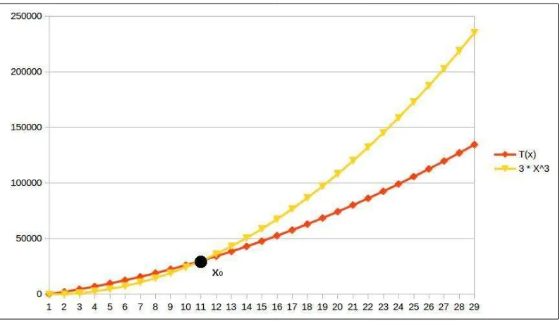
For example, Figure 1 shows an example of a function T(x) = 100x2_{+2000x+200. This}

function is O(x2_{), with some x}

0 = 11 and M = 300. The graph of 300x

2_{overcomes the}

graph of T(x) at x=11 and then stays above T(x) up to infinity. Notice that the function 300x2_{is lower than T(x) for smaller values of x, but that does not affect our conclusion.}

Figure 1. Asymptotic upper bound

To see that it's the same thing as the previous four points, first think of x₀ as the way to ensure that x is sufficiently large. I leave it up to you to prove the above four conditions from the formal definition.

I will, however, show some examples of using the formal definition:

• 5x2_{= O(x}2_{) because we can say, for example, x}

0 = 10 and M = 10 and thus f(x)

< Mg(x) whenever x > x₀, that is, 5x2_{< 10x}2_{whenever x > 10.}

• It is also true that 5x2_{= O(x}3_{) because we can say, for example, x}

0 = 10 and M

= 10 and thus f(x) < Mg(x) whenever x > x₀, that is, 5x2_{< 10x}3_{whenever x >}

(28)

• How about the function f(x) = 5x2_{- 10x + 3}? We can easily see that when _{x is}

sufficiently large, 5x2_{will far surpass the term 10x. To prove my point, I can}

simply say x>5, 5x2_{> 10x. Every time we increment x by one, the increment}

in 5x2_{is 10x + 1 and the increment in 10x is just a constant, 10. 10x+1 > 10 for}

Now, we have it true for n=0, that is, a0 = O(1). This means, by our last conclusion, a₁x + a₀ = O(x). This means, by the same logic, a₂ x2_{+ a}

1x + a0 = O(x

2_{), and so}

(29)

Asymptotic upper bound of an algorithm

Okay, so we figured out a way to sort of abstractly specify an upper bound on a function that has one argument. When we talk about the running time of a program, this argument has to contain information about the input. For example, in our algorithm, we can say, the execution time equals O(power). This scheme of specifying the input directly will work perfectly fine for all programs or algorithms solving the same problem because the input will be the same for all of them. However, we might want to use the same technique to measure the complexity of the problem itself: it is the complexity of the most efficient program or algorithm that can solve the problem. If we try to compare the complexity of different problems, though, we will hit a wall because different problems will have different inputs. We must specify the running time in terms of something that is common among all problems, and that something is the size of the input in bits or bytes. How many bits do we need to express the argument, power, when it's sufficiently large? Approximately log₂ (power). So, in specifying the running time, our function needs to have an input that is of the size log₂ (power) or lg (power). We have seen that the running time of our algorithm is proportional to the power, that is, constant times power, which is constant times 2 lg(power) = O(2x),where x= lg(power), which is the the size of the input.

Asymptotic lower bound of a function

Sometimes, we don't want to praise an algorithm, we want to shun it; for example, when the algorithm is written by someone we don't like or when some algorithm is really poorly performing. When we want to shun it for its horrible performance, we may want to talk about how badly it performs even for the best input. An a symptotic lower bound can be defined just like how greater-than-or-equal-to can be defined in terms of less-than-or-equal-to.

A function f(x) = Ω(g(x)) if and only if g(x) = O(f(x)). The following list shows a few examples:

• Since x3_{= O(x}3_{), x}3 = Ω(x3₎

• Since x3_{= O(5x}3_{), 5x}3 = Ω(x3₎

• Since x3_{= O(5x}3_{- 25x}2_{+ 1), 5x}3_{- 25x}2 + 1 = Ω(x3₎

• Since x3_{= O(x}4_{), x}4_{= O(x}3₎

(30)

The preceding definition was introduced by Donald Knuth, which was a stronger and more practical definition to be used in computer science. Earlier, there was a different definition of the lower bound Ω that is more complicated to understand and covers a few more edge cases. We will not talk about edge cases here.

While talking about how horrible an algorithm is, we can use an asymptotic lower bound of the best case to really make our point. However, even a criticism of the worst case of an algorithm is quite a valid argument. We can use an asymptotic lower bound of the worst case too for this purpose, when we don't want to find out an asymptotic tight bound. In general, the asymptotic lower bound can be used to show a minimum rate of growth of a function when the input is large enough in size.

Asymptotic tight bound of a function

There is another kind of bound that sort of means equality in terms of asymptotic complexity. A theta bound is specified as f(x) = Ͽ(g(x)) if and only if f(x) = O(g(x)) and f(x) = Ω(g(x)). Let's see some examples to understand this even better:

• Since 5x3_=O(x3_{) and also 5x}3=Ω(x3_{), we have 5x}3₌Ͽ_(x3₎

• Since 5x3_{+ 4x}2_=O(x3_{) and 5x}3_{+ 4x}2=Ω(x3_{), we have 5x}3_{+ 4x}2_=O(x3₎

• However, even though 5x3_{+ 4x}2_=O(x4), since it is not Ω(x4_{), it is also}

not Ͽ(x4₎

• Similarly, 5x3_{+ 4x}2_{is not}Ͽ_(x2_{) because it is not O(x}2₎

In short, you can ignore constant multipliers and lower order terms while

determining the tight bound, but you cannot choose a function which grows either faster or slower than the given function. The best way to check whether the bound is right is to check the O and the condition separately, and say it has a theta bound only if they are the same.

(31)

In some cases, we try to find the average case complexity, especially when the upper bound really happens only in the case of an extremely pathological input. But since the average must be taken in accordance with the probability distribution of the input, it is not just dependent on the algorithm itself. The bounds themselves are just bounds for particular functions and not for algorithms. However, the total running time of an algorithm can be expressed as a grand function that changes it's formula as per the input, and that function may have different upper and lower bounds. There is no sense in talking about an asymptotic average bound because, as we discussed, the average case is not just dependent on the algorithm itself, but also on the probability distribution of the input. The average case is thus stated as a function that would be a probabilistic average running time for all inputs, and, in general, the asymptotic upper bound of that average function is reported.

Optimization of our algorithm

Before we dive into actually optimizing algorithms, we need to first correct our algorithm for large powers. We will use some tricks to do so, as described below.

Fixing the problem with large powers

Equipped with all the toolboxes of asymptotic analysis, we will start optimizing our algorithm. However, since we have already seen that our program does not work properly for even moderately large values of power, let's first fix that. There are two ways of fixing this; one is to actually give the amount of space it requires to store all the intermediate products, and the other is to do a trick to limit all the intermediate steps to be within the range of values that the long datatype can support. We will use binomial theorem to do this part.

As a reminder, binomial theorem says (x+y)n_{= x}n₊n_C

is that all the coefficients are integers. Suppose, r is the remainder when we divide a by b. This makes a = kb + r true for some positive integer k. This means r = a-kb, and rn

Note that apart from the first term, all other terms have b as a factor. Which means that we can write rn_{= a}n + bM for some integer M. If we divide both sides by b now

and take the remainder, we have rn_{% b = a}n_{% b, where % is the Java operator for}

(32)

The idea now would be to take the remainder by the divisor every time we raise the power. This way, we will never have to store more than the range of the remainder:

public static long computeRemainderCorrected(long base, long power, long divisor){

long baseRaisedToPower = 1; for(long i=1;i<=power;i++){ baseRaisedToPower *= base; baseRaisedToPower %= divisor; }

return baseRaisedToPower; }

This program obviously does not change the time complexity of the program; it just fixes the problem with large powers. The program also maintains a constant space complexity.

Improving time complexity

The current running time complexity is O(2x_{), where x is the size of the input as we}

have already computed. Can we do better than this? Let's see.

What we need to compute is (basepower_{) % divisor. This is, of course, the same as}

(base2₎power/2_{% divisor. If we have an even power, we have reduced the number of}

operations by half. If we can keep doing this, we can raise the power of base by 2n_in

just n steps, which means our loop only has to run lg(power) times, and hence, the complexity is O(lg(2x_{)) = O(x), where x is the number of bits to store power. This is a}

substantial reduction in the number of steps to compute the value for large powers.

However, there is a catch. What happens if the power is not divisible by 2? Well, then we can write (basepower_{)% divisor = (base ((base}power-1_{))%divisor = (base ((base}2₎power-1_)%divisor,

and power-1 is, of course, even and the computation can proceed. We will write up this code in a program. The idea is to start from the most significant bit and move towards less and less significant bits. If a bit with 1 has n bits after it, it represents multiplying the result by the base and then squaring n times after this bit. We accumulate this squaring by squaring for the subsequent steps. If we find a zero, we keep squaring for the sake of accumulating squaring for the earlier bits:

public static long computeRemainderUsingEBS(long base, long power, long divisor){

(33)

First reverse the bits of our power so that it is easier to access them from the least important side, which is more easily accessible. We also count the number of bits for later use:

while(power>0){

powerBitsReversed <<= 1;

powerBitsReversed += power & 1; power >>>= 1;

numBits++; }

Now we extract one bit at a time. Since we have already reversed the order of bit, the first one we get is the most significant one. Just to get an intuition on the order, the first bit we collect will eventually be squared the maximum number of times and hence will act like the most significant bit:

while (numBits-->0){

if(powerBitsReversed%2==1){

baseRaisedToPower *= baseRaisedToPower * base; }else{

baseRaisedToPower *= baseRaisedToPower; }

baseRaisedToPower %= divisor; powerBitsReversed>>>=1; }

return baseRaisedToPower; }

We test the performance of the algorithm; we compare the time taken for the same computation with the earlier and final algorithms with the following code:

public static void main(String [] args){

System.out.println(computeRemainderUsingEBS(13, 10_000_000, 7));

long startTime = System.currentTimeMillis(); for(int i=0;i<1000;i++){

computeRemainderCorrected(13, 10_000_000, 7); }

long endTime = System.currentTimeMillis(); System.out.println(endTime - startTime);

startTime = System.currentTimeMillis(); for(int i=0;i<1000;i++){

computeRemainderUsingEBS(13, 10_000_000, 7); }

(34)

The first algorithm takes 130,190 milliseconds to complete all 1,000 times execution on my computer and the second one takes just 2 milliseconds to do the same. This clearly shows the tremendous gain in performance for a large power like 10 million. The algorithm for squaring the term repeatedly to achieve exponentiation like we did is called... well, exponentiation by squaring. This example should be able to motivate you to study algorithms for the sheer obvious advantage it can give in improving the performance of computer programs.

Summary

In this chapter, you saw how we can think about measuring the running time of and the memory required by an algorithm in seconds and bytes, respectively. Since this depends on the particular implementation, the programming platform, and the hardware, we need a notion of talking about running time in an abstract way. Asymptotic complexity is a measure of the growth of a function when the input is very large. We can use it to abstract our discussion on running time. This is not to say that a programmer should not spend any time to make a run a program twice as fast, but that comes only after the program is already running at the minimum asymptotic complexity.

We also saw that the asymptotic complexity is not just a property of the problem at hand that we are trying to solve, but also a property of the particular way we are solving it, that is, the particular algorithm we are using. We also saw that two programs solving the same problem while running different algorithms with different asymptotic complexities can perform vastly differently for large inputs. This should be enough motivation to study algorithms explicitly.

(35)

(36)

Cogs and Pulleys – Building

Blocks

We discussed algorithms in the previous chapter, but the title of the book also includes the term "data structure." So what is a data structure? A data structure is an organization of data in memory that is generally optimized so it can be used by a particular algorithm. We have seen that an algorithm is a list of steps that leads to a desired outcome. In the case of a program, there is always some input and output. Both input and output contain data and hence must be organized in some way or another. Therefore, the input and output of an algorithm are data structures. In fact, all the intermediate states that an algorithm has to go through must also be stored in some form of a data structure. Data structures don't have any use without algorithms to manipulate them, and algorithms cannot work without data structures. It's

because this is how they get input and emit output or store their intermediate states. There are a lot of ways in which data can be organized. Simpler data structures are also different types of variables. For example, int is a data structure that stores one 4-byte integer value. We can even have classes that store a set of specific types of values. However, we also need to think about how to store a collection of a large number of the same type of values. In this book, we will spend the rest of the time discussing a collection of values of the same type because how we store a collection determines which algorithm can work on them. Some of the most common ways of storing a collection of values have their own names; we will discuss them in this chapter. They are as follows:

• Arrays • Linked lists

(37)

These are the basic building blocks that we will use to build more complex data structures. Even if we don't use them directly, we will use their concepts.

Arrays

If you are a Java programmer, you must have worked with arrays. Arrays are the basic storage mechanisms available for a sequence of data. The best thing about arrays is that the elements of an array are collocated sequentially and can be accessed completely and randomly with single instructions.

The traversal of an array element by an element is very simple. Since any element can be accessed randomly, you just keep incrementing an index and keep accessing the element at this index. The following code shows both traversal and random access in an array:

System.out.println(anIntArray[i]); }

}

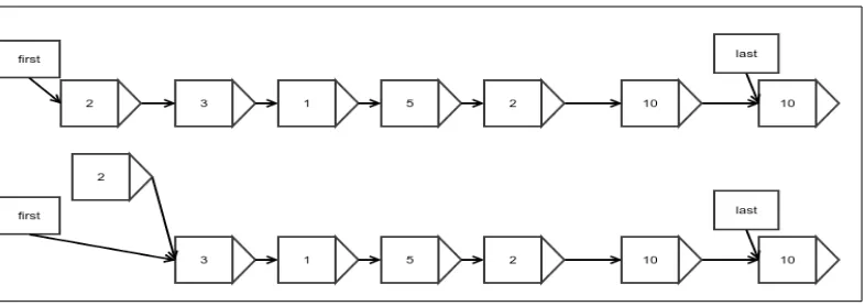
Insertion of elements in an array

(38)

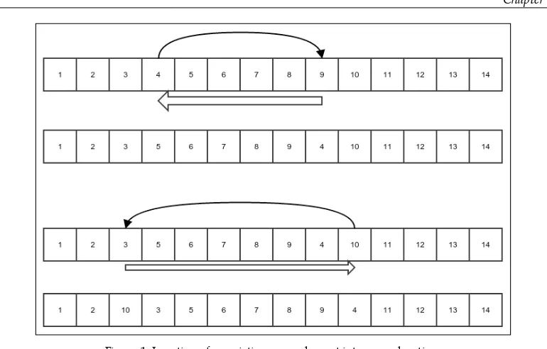
Figure 1: Insertion of an existing array element into a new location

The preceding figure explains what we mean by this operation. The thin black arrows show the movement of the element that is being reinserted, and the thick white arrow shows the shift of the elements of the array. In each case, the bottom figure shows the array after the reinsertion is done. Notice that the shifting is done either to the left or right, depending on what the start and end index are. Let's put this in code:

public static void insertElementAtIndex(int[] array, int startIndex, int targetIndex){

int value = array[startIndex]; if(startIndex==targetIndex){ return;

}else if(startIndex < tarGetIndex){

for(int i=startIndex+1;i<=targetIndex;i++){ array[i-1]=array[i];

}

array[targetIndex]=value; }else{

for(int i=startIndex-1;i>=targetIndex;i--){ array[i+1]=array[i];

}

(39)

What would be the running time complexity of the preceding algorithm? For all our cases, we will only consider the worst case. When does an algorithm perform worst? To understand this, let's see what the most frequent operation in an algorithm is. It is of course the shift that happens in the loop. The number of shifts become maximum when startIndex is at the beginning of the array and targetIndex at the end or vice versa. This is when all but one element has to be shifted one by one. The running time in this case must be some constant times the number of elements of the array plus some other constant to account for the non-repeating operations. So it is T(n) = K(n-1)+C for some constants K and C, where n is the number of elements in the array and T(n) is the running time of the algorithm. This can be expressed as follows:

T(n) = K(n-1)+C = Kn + (C-K)

The following steps explain the expression:

1. As per rule 1 of the definition of big O, T(n) = O(Kn + (C-K)). 2. As per rule 3, T(n) = O(Kn).

3. We know |-(C-K)| < |Kn + (C-K)| is true for sufficiently large n. Therefore, as per rule 3, since T(n) = O(Kn + (C-K)), it means T(n) = O(Kn + (C-K) + (-(C-K))), that is, T(n) = O(Kn).

4. And, finally, as per rule 2, T(n) = O(n).

Now since the array is the major input in the algorithm, the size of the input is represented by n. So we will say, the running time of the algorithm is O(n), where n is the size of the input.

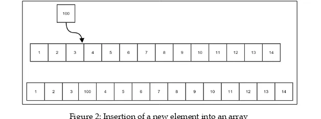
Insertion of a new element and the process of

appending it

Now we move on to the process of insertion of a new element. Since arrays are fixed in size, insertion requires us to create a new array and copy all the earlier elements into it. The following figure explains the idea of an insertion made in a new array:

(40)

The following code does exactly that:

public static int [] insertExtraElementAtIndex(int[] array, int index, int value){

int [] newArray = new int[array.length+1];

First, you copy all the elements before the targeted position as they are in the original array:

for(int i=0;i<index;i++){ newArray[i] = array[i]; }

Then, the new value must be put in the correct position:

newArray[index]=value;

In the end, copy the rest of the elements in the array by shifting their position by one:

for(int i=index+1;i<newArray.length;i++){ newArray[i]=array[i-1];

}

return newArray; }

When we have the code ready, appending it would mean just inserting it at the end, as shown in the following code:

public static int[] appendElement(int[] array, int value){

return insertExtraElementAtIndex(array, array.length, value); }

(41)

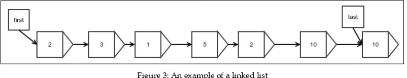
Linked list

Arrays are great for storing data. We have also seen that any element of an array can be read in O(1) time. But arrays are fixed in size. Changing the size of an array means creating a new array and copying all the elements to the original array. The simplest recourse to the resizing problem is to store each element in a different object and then hold a reference in each element to the next element. This way, the process of adding a new element will just involve creating the element and attaching it at the end of the last element of the original linked list. In another variation, the new element can be added to the beginning of the existing linked list:

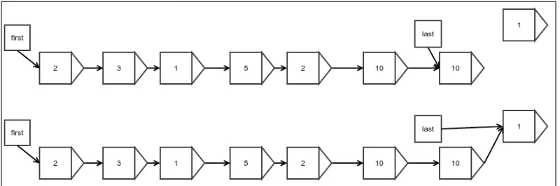
Figure 3: An example of a linked list

Figure 3 shows an example of a linked list. The arrows represent a reference. Each element is stored in a wrapper object that also holds a reference to the next element wrapper. There are two additional references to the first and last elements, which are required for any operation to start. The last reference is optional, but it improves the performance of appending to the end vastly, as we shall see.

To begin the discussion, let's create a linked list node in the following way:

public class LinkedList<E> implements Iterable<E>, Visualizable {

First, we create a Node class inside the LinkedList class, which will act as a wrapper for the elements and also hold the reference to the next node:

protected static class Node<E> { protected E value;

protected Node next;

public String toString(){ return value.toString(); }

}

int length = 0;

(42)

Then, we must have references for the first and last elements:

Node<E> first; Node<E> last;

Finally, we create a method called getNewNode() that creates a new empty node. We will need this if we want to use a different class for a node in any of the subclasses:

protected Node<E> getNewNode() { Node<E> node = new Node<>();

lastModifiedNode = new Node[]{node}; return node;

} }

At this point, the unfinished class LinkedList will not be able to store any element; let's see how to do this, though. Notice that we have implemented the Iterable interface. This will allow us to loop through all the elements in an advanced for loop.

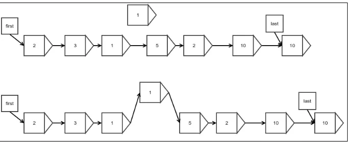
Appending at the end

Appending at the end is achieved by simply creating a link from the last element of the original linked list to the new element that is being appended and then

reassigning the reference to the last element. The second step is required because the new element is the new last element. This is shown in the following figure:

(43)

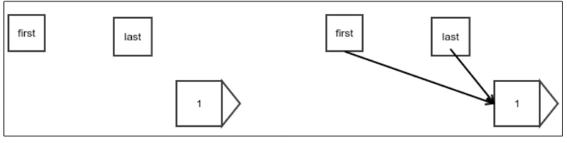
There is a small difference when you append an element to a linked list that is empty to start with. At this point, the first and last references are null, and this case must be handled separately. The following figure explains this case:

Figure 5: Appending to an empty linked list

We will achieve this by using the following simple code as is. We return the node that has just been added. This is helpful to any class that is extending this class. We will do the same in all cases, and we will see the use of this while discussing doubly linked lists:

public Node<E> appendLast(E value) { Node node = getNewNode();

node.value = value;

We try to update the reference of the current last node only if the list is not empty:

if (last != null) last.next = node;

Then, we must update the last reference as the new element is not going to be the last element:

last = node;

Finally, if the list is empty, the new element must also be the first new element and we must update the first reference accordingly, as shown in the preceding figure:

if (first == null) { first = node; }

(44)

Notice that we also keep track of the current length of the list. This is not essential, but if we do this, we do not have to traverse the entire list just to count how many elements are in the list.

Now, of course, there is this important question: what is the time complexity of appending to a linked list? Well, if we do it the way we have done it before—that is, by having a special reference to the last element—we don't need any loop, as we can see in the code. If the program does not have any loops, all operations would be one-time operations, hence everything is completed in constant one-time. You can verify that a constant function has this complexity: O(1). Compare this with what was appended at the end of an array. It required the creation of a new array and also had O(n) complexity, where n was the size of the array.

Insertion at the beginning

Inserting an element at the beginning of a list is very similar to appending it at the end. The only difference is that you need to update the first reference instead of the last reference:

public Node<E> appendFirst(E value) { Node node = getNewNode();

node.value = value; node.next = first; first = node; if (length == 0) last = node; length++;

(45)

Insertion at an arbitrary position

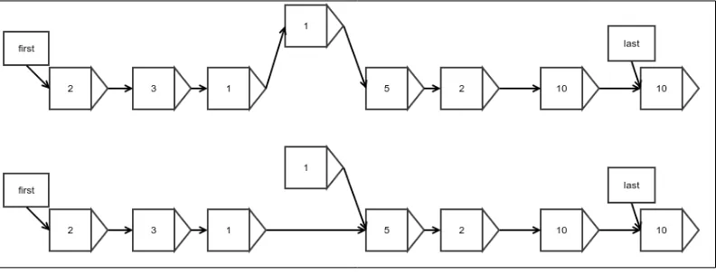
Insertion at an arbitrary position can be achieved in the same way we perform an insertion in the first element, except that we update the reference of the previous element instead of the first reference. There is, however, a catch; we need to find the position where we need to insert the element. There is no way to find it other than to start at the beginning and walk all the way to the correct position while counting each node we step on.

Figure 6: Insertion of an arbitrary element into a linked list

We can implement the idea as follows:

public Node<E> insert(int index, E value) { Node<E> node = getNewNode();

First, we take care of the special cases:

if (index < 0 || index > length) {

throw new IllegalArgumentException("Invalid index for insertion");

} else if (index == length) { return appendLast(value); } else if (index == 0) { return appendFirst(value); } else {

As mentioned earlier, we walk all the way to the desired position while counting the nodes, or in this case, counting the index in the opposite direction:

Node<E> result = first; while (index > 1) { index--;

(46)

Finally, we update the references:

node.value = value; node.next = result.next; result.next = node; length++;

return node; }

}

What is the complexity of this algorithm? There is a loop that must run as many times as the index. This algorithm seems to have a running time that is dependent on the value of the input and not just its size. In this case, we are only interested in the worst case. What is the worst case then? It is when we need to step on all the elements of the list, that is, when we have to insert the element at the end of the list, except for the last element. In this case, we must step on n-1 elements to get there and do some constant work. The number of steps would then be T(n) = C(n-1)+K for some constants C and K. So, T(n) = O(n).

Looking up an arbitrary element

Finding the value of an arbitrary element has two different cases. For the first and last element, it is simple. Since we have direct references to the first and last element, we just have to traverse that reference and read the value inside it. I leave this for you to see how it could be done.

However, how do you read an arbitrary element? Since we only have forward references, we must start from the beginning and walk all the way, traversing references while counting steps until we reach the element we want.

Let's see how we can do this:

public E findAtIndex(int index) {

We start from the first element:

Node<E> result = first; while (index >= 0) { if (result == null) {

(47)

When the index is 0, we would have finally reached the desired position, so we return:

return result.value; } else {

If we are not there yet, we must step onto the next element and keep counting:

index--;

result = result.next; }

}

return null; }

Here too, we have a loop inside that has to run an index a number of times. The worst case is when you just need to remove one element but it is not the last one; the last one can be found directly. It is easy to see that just like you insert into an arbitrary position, this algorithm also has running time complexity of O(n).

Figure 7: Removing an element in the beginning

Removing an element in the beginning means simply updating the reference to the first element with that of the next element. Note that we do not update the reference in the element that has just been removed because the element, along with the reference, would be garbage-collected anyway:

public Node<E> removeFirst() { if (length == 0) {

(48)

Assign the reference to the next element:

Node<E> origFirst = first; first = first.next;

length--;

If there are no more elements left, we must also update the last reference:

if (length == 0) { last = null; }

return origFirst; }

Removing an arbitrary element

Removing an arbitrary element is very similar to removing an element from the beginning, except that you update the reference held by the previous element instead of the special reference named first. The following figure shows this:

Figure 8: Removing an arbitrary element

Notice that only the link in the linked list is to be reassigned to the next element. The following code does what is shown in the preceding figure:

(49)

Of course, removing the first element is a special case:

if (index == 0) {

Node<E> nodeRemoved = first; removeFirst();

return nodeRemoved; }

First, find out the element just before the one that needs to be removed because this element would need its reference updated:

Node justBeforeIt = first; while (--index > 0) {

justBeforeIt = justBeforeIt.next; }

Update the last reference if the last element is the one that is being removed:

Node<E> nodeRemoved = justBeforeIt.next; if (justBeforeIt.next == last) {

last = justBeforeIt.next.next; }

Update the reference held by the previous element:

justBeforeIt.next = justBeforeIt.next.next; length--;

return nodeRemoved; }

It is very easy to see that the running time worst case complexity of this algorithm is O(n)—which is similar to finding an arbitrary element—because this is what needs to be done before removing it. The operation of the actual removal process itself requires only a constant number of steps.

Iteration

Since we are working in Java, we prefer to implement the Iterable interface. It lets us loop through the list in a simplified for loop syntax. For this purpose, we first have to create an iterator that will let us fetch the elements one by one:

protected class ListIterator implements Iterator<E> { protected Node<E> nextNode = first;

(50)

public boolean hasNext() { return nextNode != null; }

@Override

public E next() { if (!hasNext()) {

throw new IllegalStateException(); }

Node<E> nodeToReturn = nextNode; nextNode = nextNode.next;

return nodeToReturn.value; }

}

The code is self-explanatory. Every time it is invoked, we move to the next element and return the current element's value. Now we implement the iterator method of the Iterable interface to make our list an iterable:

@Override

public Iterator<E> iterator() { return new ListIterator(); }

This enables us to use the following code:

for(Integer x:linkedList){ System.out.println(x); }

The preceding code assumes that the variable linkedList was

(51)

Doubly linked list

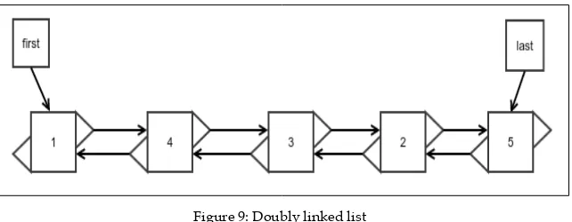
Did you notice that there is no quick way to remove the element from the end of a linked list? This is because even if there is a quick way to find the last element, there is no quick way to find the element before it whose reference needs to be updated. We must walk all the way from the beginning to find the previous element. Well then, why not just have another reference to store the location of the last but one element? This is because after you remove the element, how would you update the reference otherwise? There would be no reference to the element right before that. What it looks like is that to achieve this, we have to store the reference of all the previous elements up to the beginning. The best way to do this would be to store the reference of the previous element in each of the elements or nodes along with the reference to the next element. Such a linked list is called a doubly linked list since the elements are linked both ways:

Figure 9: Doubly linked list

We will implement a doubly linked list by extending our original linked list because a lot of the operations would be similar. We can create the barebones class in the following manner:

public class DoublyLinkedList<E> extends LinkedList<E> {

We create a new Node class extending the original one and adding a reference for the previous node:

protected static class DoublyLinkedNode<E> extends Node<E> { protected DoublyLinkedNode<E> prev;

}

Of course, we need to override the getNode() method to use this node:

@Override

protected Node<E> getNewNode() { return new DoublyLinkedNode<E>(); }

(52)

Insertion at the beginning or at the end

Insertion at the beginning is very similar to that of a singly linked list, except that we must now update the next node's reference for its previous node. The node being inserted does not have a previous node in this case, so nothing needs to be done:

public Node<E> appendFirst(E value) {

Node<E> node = super.appendFirst(value); if (first.next != null)

((DoublyLinkedNode<E>) first.next).prev = (DoublyLinkedNode<E>) first;

return node; }

Pictorially, it can be visualized as shown in the following figure:

Figure 10: Insertion at the beginning of a doubly linked list

Appending at the end is very similar and is given as follows:

public Node<E> appendLast(E value) {

DoublyLinkedNode<E> origLast = (DoublyLinkedNode<E>) this.last;

Node<E> node = super.appendLast(value);

If the original list were empty, the original last reference would be null:

if (origLast == null) {

origLast = (DoublyLinkedNode<E>) first; }

(53)

The complexity of the insertion is the same as that of a singly linked list. In fact, all the operations on a doubly linked list have the same running time complexity as that of a singly linked list, except the process of removing the last element. We will thus refrain from stating it again until we discuss the removal of the last element. You should verify that the complexity stays the same as with a singly linked list in all other cases.

Insertion at an arbitrary location

As with everything else, this operation is very similar to the process of making an insertion at an arbitrary location of a singly linked list, except that you need to update the references for the previous node.

Figure 11: Insertion at an arbitrary location of a doubly linked list

The following code does this for us:

public Node<E> insert(int index, E value) {

(54)

In the case of the first and last element, our overridden methods are invoked anyway. Therefore, there is no need to consider them again:

if(index!=0 && index!=length) { if (inserted.next != null) {

This part needs a little bit of explaining. In Figure 11, the node being inserted is 13. Its previous node should be 4, which was originally the previous node of the next node 3:

inserted.prev = ((DoublyLinkedNode<E>) inserted.next).prev;

The prev reference of the next node 3 must now hold the newly inserted node 13:

((DoublyLinkedNode<E>) inserted.next).prev = inserted; }

}

return inserted; }

Removing the first element

Removing the first element is almost the same as that for a singly linked list. The only additional step is to set the prev reference of the next node to null. The following code does this:

public Node<E> removeFirst() { super.removeFirst(); if (first != null) {

((DoublyLinkedNode<E>) first).prev = null; }

(55)

The following figure shows what happens. Also, note that finding an element does not really need an update:

Figure 12: Removal of the first element from a doubly linked list

There can be an optimization to traverse backward from the last element to the first in case the index we are looking for is closer toward the end; however, it does not change the asymptotic complexity of the find operation. So we leave it at this stage. If interested, you would be able to easily figure out how to do this optimization.

Removing an arbitrary element

(56)

Figure 13: Removal of an arbitrary element from a doubly linked list

The following code will help us achieve this:

public Node<E> removeAtIndex(int index) { if(index<0||index>=length){

throw new NoSuchElementException(); }

This is a special case that needs extra attention. A doubly linked list really shines while removing the last element. We will discuss the removeLast() method in the next section:

Java 9 Data Structures and Algorithms A step by step guide to data structures and algorithms pdf pdf

Java 9 Data Structures and

Algorithms

A step-by-step guide to data structures and algorithms

Debasish Ray Chawdhuri

Java 9 Data Structures and Algorithms

Credits

About the Author

Debasish Ray Chawdhuri

About the Reviewer

Miroslav Wengner

www.PacktPub.com

eBooks, discount offers, and more

Why subscribe?

Customer Feedback

Table of Contents

Preface vii

Chapter 1: Why Bother? – Basic

1

Chapter 2: Cogs and Pulleys – Building Blocks

15

Chapter 3: Protocols – Abstract Data Types

41

Chapter 4: Detour – Functional Programming

57

Chapter 5:

Efficient Searching – Binary Search and Sorting

91

Chapter 6:

Efficient Sorting – quicksort and mergesort

115

Chapter 7: Concepts of Tree

135

Chapter 8: More About Search – Search Trees and Hash Tables

155

Chapter 9: Advanced General Purpose Data Structures

195

Chapter 10: Concepts of Graph

225

Chapter 11: Reactive Programming

281

Preface

What this book covers

What you need for this book

Who this book is for

Conventions

Reader feedback

Customer support

Downloading the example code

Downloading the color images of this book

Errata

Piracy

Questions

Why Bother? – Basic

The performance of an algorithm

Best case, worst case and the average case

complexity

Analysis of asymptotic complexity

Asymptotic upper bound of a function

Asymptotic upper bound of an algorithm

Asymptotic lower bound of a function

Asymptotic tight bound of a function

Optimization of our algorithm

Fixing the problem with large powers

Improving time complexity

Summary

Cogs and Pulleys – Building

Blocks

Arrays

Insertion of elements in an array

Insertion of a new element and the process of

appending it

Linked list

Appending at the end

Insertion at the beginning

Insertion at an arbitrary position

Looking up an arbitrary element

Removing an arbitrary element

Iteration

Doubly linked list