Assessment of temporal and spatial changes of future climate in the
Jhelum river basin, Pakistan and India
Rashid Mahmood
a,c,n, Mukand S Babel
b, Shaofeng JIA
a,caDepartment of Irrigation and Drainage, Faculty of Agricultural Engineering and Technology, University of Agriculture, Faisalabad, Pakistan bWater Engineering and Management, Asian Institute of Technology, Pathumthani, Thailand
cInstitute of Geographic Science and Natural Resources Research / Key Laboratory of Water Cycle and Related Land Surface Processes, Chinese Academy of Sciences, Beijing, 100101, China
a r t i c l e
i n f o
The present study investigated future temporal and spatial changes in maximum temperature, minimum temperature, and precipitation in two sub-basins of the Jhelum River basin—the Two Peak Precipitation basin (TPPB) and the One Peak Precipitation basin (OPPB)—and in the Jhelum River basin on the whole, using the statistical downscaling model, SDSM. The Jhelum River is one of the biggest tributaries of the Indus River basin and the main source of water for Mangla reservoir, the second biggest reservoir in Pakistan.
An advanced interpolation method, kriging, was used to explore the spatial variations in the study area. Validation results showed a better relationship between simulated and observed monthly time series as well as between seasonal time series relative to daily time series, with an averageR2of 0.92
– 0.97 for temperature and 0.22–0.62 for precipitation.
Mean annual temperature was projected to rise significantly in the entire basin under two emission scenarios of HadCM3 (A2 and B2). However, these changes in mean annual temperature were predicted to be higher in the TPPB than the OPPB. On the other hand, mean annual precipitation showed a distinct increase in the TPPB and a decrease in the OPPB under both scenarios.
In the case of seasonal changes, spring in the TPPB and autumn in the OPPB were projected to be the most affected seasons, with an average increase in temperature of 0.43–1.7°C in both seasons relative to baseline period. Summer in the TPPB and autumn in the OPPB were projected to receive more pre-cipitation, with an average increase of 4–9% in both seasons, and winter in the TPPB and spring in the OPPB were predicted to receive 2–11% less rainfall under both future scenarios, relative to the baseline period.
In the case of spatial changes, some patches of the basin showed a decrease in temperature but most areas of the basin showed an increase. During the 2020s (2011–2040), about half of the basin showed a decrease in precipitation. However, in the 2080s (2071–2099), most parts of the basin were projected to have decreased precipitation under both scenarios.
&2015 The Authors. Published by Elsevier B.V. This is an open access article under the CC BY license (http://creativecommons.org/licenses/by/4.0/).
1. Introduction
The concentration of CO2and other greenhouse gases has been
increasing dramatically since 1950, mostly because of in-dustrialization (Gebremeskel et al., 2005). This increase has caused a global energy imbalance and has increased global warming. Ac-cording to the Fifth Assessment Report of the Intergovernmental
Panel on Climate Change (IPCC), global (land and ocean) mean surface temperature as calculated by a linear trend over the period 1880–2012, show a warming of 0.85°C (0.65–1.06°C). An alarming increase of 0.78 (0.72–0.85)°C has been observed for the period of 2003–2012 with respect to 1850–1900. Global mean surface tem-peratures is projected to increase by 0.3–1.7°C, 1.1 to 2.6°C, 1.4– 3.1°C, and 2.6–4.8°C under RCP2.6, RCP4.5, RCP6.0 and RCP8.5, respectively, for 2081–2100 relative to 1986–2005 (IPCC, 2013).
This global warming can disturb the hydrological cycle of the world, and can pose problems for public health, industrial and municipal water demand, water energy exploitation, and the ecosystem (Chu et al., 2010;Zhang et al., 2011).
Contents lists available atScienceDirect
journal homepage:www.elsevier.com/locate/wace
Weather and Climate Extremes
http://dx.doi.org/10.1016/j.wace.2015.07.002
2212-0947/&2015 The Authors. Published by Elsevier B.V. This is an open access article under the CC BY license (http://creativecommons.org/licenses/by/4.0/). n
Corresponding author at: Department of Irrigation and Drainage, Faculty of Agricultural Engineering and Technology, University of Agriculture, Faisalabad, Pakistan.
In the last few decades, Global Climate Models (GCMs)—the most advanced and numerical-based coupled models representing the global climate system—have been used to examine future changes in climate variables such as temperature, precipitation, and evaporation (Fowler et al., 2007). However, their outputs are temporally and spatially very coarse (Gebremeskel et al., 2005), which makes them useful only at continental and global levels. Their application at local/regional levels, such as at the basin and sub-basin scales, to assess the impacts of climate change on the environment and hydrological cycle, is problematic due to a clear resolution mismatch (Hay et al., 2000;Wilby et al., 2000). That is, GCMs cannot give a realistic presentation of local or regional scales due to parameterization limitations (Benestad et al., 2008). The local and regional scales are defined as 0–50 km and 5050 km2,
respectively (Xu, 1999)
To overcome this problem, during the last two decades, many downscaling methods have been developed to make the large-scale outputs of GCMs useful at local/regional large-scales (Wetterhall et al., 2006). In the beginning, these methods were mostly im-plemented in Europe and in the USA but are now applied throughout the globe to examine changes in climate variables at the basin level (Mahmood and Babel, 2012).
Generally, downscaling techniques are divided into two main categories: Dynamical Downscaling (DD), and Statistical Down-scaling (SD). In DD, a Regional Climate Model (RCM) of high re-solution (5–50 km) (Chu et al., 2010), nested within a GCM, re-ceives inputs from the GCM and then provides high resolution outputs on a local scale. Since the RCM is dependent on the boundary conditions of a GCM, there is a greater chance that systematic errors that belong to the drivingfields of the GCM will be inherited by the RCM. In addition, simulations from RCMs are
computationally intensive, and depend upon the domain size and resolution at which the RCMs are to run, which in turn limits the number of climate projections (Fowler et al., 2007).
In contrast, SD approaches, which establish a bridge among the large-scale variables (e.g., mean sea level pressure, temperature, zonal wind, and geopotential height) and local-scale variables (e.g., observed temperature and precipitation) by creating em-pirical/statistical relationships, are computationally inexpensive and much simpler than DD (Wetterhall et al., 2006). Moreover, SD approaches offer immediate solutions for downscaling climate variables and, accordingly, they have rapidly been adopted by a wider community of scientists (Wilby et al., 2000;Fowler et al., 2007). The limitation of SD is that historical meteorological station data over a long period of time is required to establish a suitable statistical or empirical relationship with large-scale variables (Chu et al., 2010). This relationship is considered to be temporally sta-tionary, which is the main assumption of this method (Hay and Clark, 2003). In addition, SD is mainly dependent on the level of uncertainties of the parent GCM(s). DD, therefore, is a good al-ternative for SD in basins where no historical data is available (Benestad et al., 2008).
To date, many SD models have been developed for down-scaling, and among them Statistical Downscaling Model (SDSM) was selected for this study. SDSM—a combination of multiple linear regression and a stochastic weather generator—is a well-known statistical model, and is frequently used for downscaling important climate variables (e.g., temperature, precipitation, and evaporation). The downscaled variables are used to assess hydro-logical responses under changing climatic conditions (Diaz-Nieto and Wilby, 2005;Gagnon et al., 2005; Gebremeskel et al., 2005; Wilby et al., 2006). SDSM has been widely used throughout the
world in many impact assessment studies (Huang et al., 2011). Several studies (Tripathi et al., 2006; Anandhi et al., 2007; Akhtar et al., 2008;Ghosh and Mujumdar, 2008;Mujumdar and Ghosh, 2008; Akhtar et al., 2009; Ashiq et al., 2010; Goyal and Ojha, 2010;Opitz-Stapleton and Gangopadhyay, 2010) have used SD and DD techniques in South Asia. However, most of these studies have been conducted in Indian river basins. A couple of studies, such as byAkhtar et al. (2008,2009)and byAshiq et al. (2010)using DD, and a study byMahmood and Babel (2012)using SD, were conducted in Pakistan to investigate future changes in climate variables. In the study byAkhtar et al. (2008), a Regional Climate model, Providing Regional Climate for Impact Studies (PRECIS), and delta change were used to downscale mean tem-perature and precipitation in order to analyze hydrological re-sponses to climate change in the Hindukush–Karakorum– Hima-layas (HKH). However, future changes were only investigated un-der the A2 scenario and only for the period of 2071–2100. The study concluded that the simulations from PRECIS have several uncertainty sources. Ashiq et al. (2010) interpolated monthly precipitation outputs of PRECIS, run byAkhtar et al. (2008), from a coarse resolution (5050 km2) to afine one (250250 m2) using
some interpolation methods. Their study was carried out in the northwest region of the Himalayan Mountains and in the upper Indus plains of Pakistan. They also covered a small part of the Jhelum River basin, located inside Pakistan. The study’s conclusion was that systematic errors associated with an RCM cannot be re-duced by a simple interpolation methods.
Mahmood and Babel (2012)evaluated two sub-models of SDSM (annual and monthly sub-models) out of three sub-models (monthly, annual, and seasonal) in the Jhelum River basin. They concluded that the annual sub-model cannot be used to in-vestigate the intra-annual (monthly or seasonal time series)
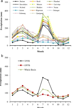
a
b
Fig. 2.Distribution of mean monthly rainfall at (a) all the weather stations and (b) in the TPPB, OPPB, and the whole Jhelum basin for 1961–1990 (the baseline period).
Table 1
Statistics of climate stations for the period of 1961-1990 in the Jhelum River basin.
Station Elevation Annual pre-cipitation (mm)
Mean Tmax (°C)
Mean Tmin (°C)
Tmean(°C)
TPPB
1 Jhelum 287 860 30.51 16.54 23.53
2 Kotli 614 1249 28.41 15.75 22.08
3 Plandri 1402 1459 22.73 11.30 17.01 4 Rawalakot 1676 1398 21.87 10.25 16.06 5 Murree 2213 1765 16.57 8.97 12.77 6 Garidopatta 814 1586 26.06 12.58 19.32 7 Muzaffarabad 702 1418 27.34 13.54 20.44 8 Balakot 995 1731 25.04 12.01 18.53
Average 1088 1341 26.21 13.50 19.85
OPPB
9 Naran 2362 1217 11.14 1.15 6.14
10 Kupwara 1609 1314 19.64 6.30 12.93 11 Gulmarg 2705 1574 11.73 1.98 6.81 12 Srinagar 1587 764 19.76 7.37 13.52 13 Qazigund 1690 1395 19.11 6.57 12.80
14 Astore 2168 564 15.48 4.06 9.77
Average 2020 1139 16.88 5.04 10.93
Whole basin 1487 1202 19.79 7.68 13.72
Tmean¼mean temperature, Tmax¼maximum temperature, Tmin¼minimum temperature
a
b
variations in climate variables (like temperature and precipitation) without Bias Correction, although SDSM was able to predict mean annual values quite well. They also concluded that the monthly sub-model is capable of examining intra-annual variations without any Bias Correction.
No studies, to the best of our knowledge, have investigated the temporal and spatial future changes in maximum temperature, minimum temperature, and precipitation under A2 and B2 sce-narios in the upper Jhelum River basin—one of the biggest tribu-taries of the Indus River basin and drains entirely into Mangla reservoir, the second biggest reservoir in Pakistan.
In the present study, the monthly sub-model of SDSM, as re-commended by Mahmood and Babel (2012), was applied to
analyze the temporal and spatial changes in maximum tempera-ture, minimum temperatempera-ture, and precipitation for the period of 2011–2099, under A2 and B2 scenarios of HadCM3. Since the study area is mountainous and has great altitudinal variations as shown inFig. 1, an advanced spatial interpolation method, Kriging, was used to explore the spatial variability in the basin. For the sake of detailed analysis, the whole Jhelum basin was divided into two sub-basins, based on precipitation regimes. This study can be a guide for researchers who wish to apply statistical downscaling methods on mountainous regions in the Upper Indus basin, which is highly influenced by the monsoons.
2. Study area and data description
2.1. Study area
The upper Jhelum River basin—located in Pakistan and India— stretches between 73–75.62°E and 33–35°N, as shown inFig. 1. The Jhelum River, the second biggest tributary of the Indus River system (Ahmad and Chaudhry, 1988), has a drainage area of 33,342 km2, with an elevation ranging from 235 to 6285 m. The
whole basin drains into Mangla Reservoir, constructed in 1967, which is the second biggest reservoir in Pakistan. The main pur-pose of this dam is to provide irrigation water to 6 million hectares of land. Its secondary function is to produce hydropower; it has an installed capacity of 1000 MW, contributing 6% of the country’s installed capacity (Archer and Fowler, 2008;Qamer et al., 2008). For the purposes of the present study, the basin was divided into
Table 2
NCEP predictors used in the screening process of SDSM.
Predictors Description Predictors Description
1 p_f Surface airflow strength 14 r500 500 hPa relative humidity
2 p_u Surface zonal velocity 15 p8_f 850 hPa airflow strength
3 p_v Surface meridional velocity 16 p8_u 850 hPa zonal velocity
4 p_z Surface vorticity 17 p8_v 850 hPa meridional velocity
5 p_th Surface wind direction 18 p8_z 850 hPa vorticity
6 p_zh Surface divergence 19 p8th 850 hPa wind direction
7 rhum Surface relative humidity 20 p8zh 850 hPa divergence
8 p5_f 500 hPa airflow strength 21 r850 850 hPa relative humidity
9 p5_u 500 hPa zonal velocity 22 p500 500 hPa geopotential height
10 p5_v 500 hPa meridional velocity 23 p850 850 hPa geopotential height
11 p5_z 500 hPa vorticity 24 temp Mean temperature at 2 m height
12 p5th 500 hPa wind direction 25 shum Surface specific humidity
13 p5zh 500 hPa divergence 26 mslp Mean sea level pressure
Table 3
Selected predictors and their mean absolute partial correlation coefficients during the screening process of SDSM.
Tmax Abs P.r Tmin Abs P.r Precipitation Abs P.r
TPPB temp 0.73 temp 0.82 Shum 0.21
r500 0.22 rhum 0.18 p5_v 0.14
P8_z 0.19 r500 0.12 r850 0.10
P8_z 0.32 p8_v 0.15
Mslp 0.12
OPPB temp 0.76 temp 0.79 p5_v 0.23
p_u 0.38 p_u 0.37 p8_v 0.14
p_z 0.32 p_z 0.32 p5_z 0.11
P8_z 0.25 p8_z 0.26 p8_z 0.08
r500 0.17
Words in bold are super predictors;Abs P.r is the absolute partial correlation coefficient
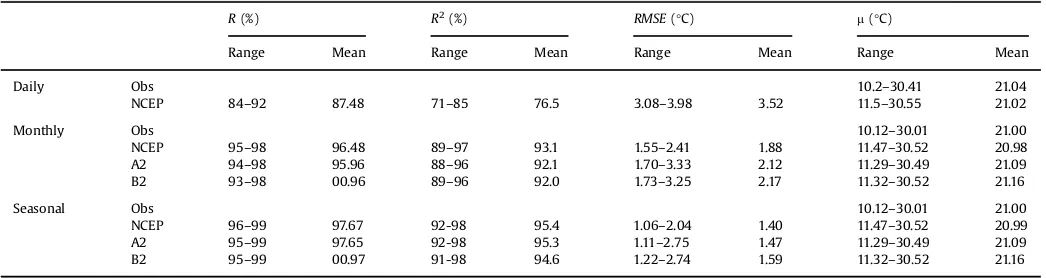
Table 4
Validation (1991-2000) of SDSM for Tmax, using daily, monthly, and seasonal time series in the Jhelum River basin.
R(%) R2(%) RMSE(
°C) m(°C)
Range Mean Range Mean Range Mean Range Mean
Daily Obs 10.2–30.41 21.04
NCEP 84–92 87.48 71–85 76.5 3.08–3.98 3.52 11.5–30.55 21.02
Monthly Obs 10.12–30.01 21.00
NCEP 95–98 96.48 89–97 93.1 1.55–2.41 1.88 11.47–30.52 20.98
A2 94–98 95.96 88–96 92.1 1.70–3.33 2.12 11.29–30.49 21.09
B2 93–98 00.96 89–96 92.0 1.73–3.25 2.17 11.32–30.52 21.16
Seasonal Obs 10.12–30.01 21.00
NCEP 96–99 97.67 92-98 95.4 1.06–2.04 1.40 11.47–30.52 20.99
A2 95–99 97.65 92-98 95.3 1.11–2.75 1.47 11.29–30.49 21.09
B2 95–99 00.97 91-98 94.6 1.22–2.74 1.59 11.32–30.52 21.16
two parts, based on the precipitation regimes of the basin, as discussed inSection 2.3.
2.2. Data description
Historical daily data of maximum temperature (Tmax), mini-mum temperature (Tmin), and precipitation (P) was collected from the Water and Power Development Authority of Pakistan (WAP-DA), Pakistan Meteorological Department (PMD), and the Indian Meteorological Department (IMD). The dataset was obtained from 14 climate stations located in the basin (Fig. 1) for the period of 1961–2000. The historical data of Kupwara, Srinagar, Gulmarg, and Qazigund was obtained from the IMD; the data of Rawlakot, Plandri, Kotli, and Naran was obtained from the WAPDA; and, the data of Muzaffarabad, Jhelum, Garidopatta, Balakot, Murree, and Astore was obtained from PMD. Some part of the daily P data for Srinagar and Qazigund for the period of 1961–1970 was acquired from the National Climate Data Center (NCDC). Although Astore and Jhelum do not lie in the upper Jhelum River basin, these sta-tions were included in the present study due to the lack of climate stations in the basin. In addition, both stations have good quality historical meteorological data. There were some missing values on some weather stations which wasfilled by multiple imputation method, using winMice software (Jacobusse, 2005)
The daily predictors of National Centers for Environmental Prediction (NCEP) for 1961–2001 and the daily predictors of HadCM3 (A2 and B2 scenarios) for 1961–2099 were collected from
a Canadian website (http://www.cccsn.ec.gc.ca/?page¼dst-sdi).
A2 and B2 are the IPCC emission scenarios of HadCM3 and are mostly used for regional impact assessment studies. These pre-dictors are specially prepared for SDSM. During the preparation, the NCEP predictors (2.5°2.5°) werefirst interpolated to the grid
resolution of HadCM3 (2.5°3.75°) to eliminate any spatial
mis-match. Then, the NCEP and HadCM3 predictors were normalized with mean and standard deviations of a long period (1961–1990) (CCCSN, 2012).
2.3. Climatic condition in the study area
The mean monthly rainfall regimes of all the climate stations used in this study for the period of 1961–1990 are shown inFig. 2 (a). Naran, Srinagar, Kupwara, Gulmarg, Astore and Qazigund cli-mate stations experience one big peak in March, and Kotli, Jhelum, Murree, Plandri, Rawlakot, Murree, Garidopatta, Muzaffarabad and Balakot experience two peaks, one small peak around March, and other big peak around July. According to the P regimes, the whole basin was divided into two sub-basins: (1) the One Peak Pre-cipitation basin (OPPB), and (2) the Two Peak PrePre-cipitation basin (TPPB). The OPPB contains most of the northeast parts of the Jhelum basin, including Srinagar, Gulmarg, Qazigund and Astore weather stations, and some of the northwest parts of the basin, including Naran and Kupwara weather stations. The TPPB consists of the southwest parts of the basin, containing Jhelum, Kotli, Plandri, Rawlakot and Murree climate stations, and the northwest
Table 5
Validation (1991–2000) of SDSM forTmin, using daily, monthly, and seasonal time series in the Jhelum River basin.
R(%) R2(%) RMSE(
°C) m(°C)
Range Mean Range Mean Range Mean Range Mean
Daily Obs 1.54–16.85 9.15
NCP 88–95 92.27 77–89 85.2 2.32–3.26 2.642 1.18–16.51 8.98
Monthly Obs 1.48–16.82 9.11
NCEP 93–99 97.49 87–98 95.1 1.09–2.41 1.45 1.13–16.47 8.94
A2 93–98 96.81 86–97 93.7 1.23–3.15 1.75 1.08–16.51 9.05
B2 93–98 96.59 86–97 93.3 1.26–3.16 1.82 1.10–16.52 9.06
Seasonal Obs 1.48–16.82 9.11
NCEP 95–99 98.37 90–99 96.8 0.56–2.00 1.045 1.13–16.47 8.94
A2 94–99 98.20 89–99 96.4 0.60–2.50 1.182 1.08–16.51 9.05
B2 94–99 97.90 88–99 95.9 0.63–2.58 1.268 1.10–16.52 9.06
R¼Correlation coefficient,R2¼Coefficient of determination,RMSE¼Root mean square error, andm¼mean
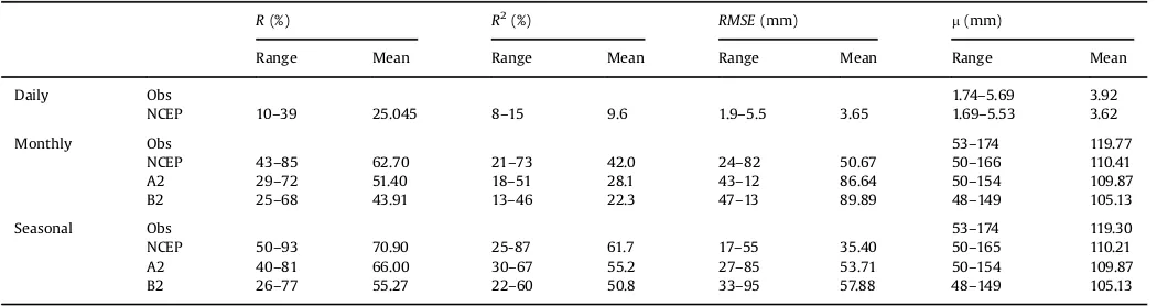
Table 6
Validation (1991–2000) of SDSM for precipitation, using daily, monthly, and seasonal time series in the Jhelum River basin.
R(%) R2(%) RMSE(mm)
m(mm)
Range Mean Range Mean Range Mean Range Mean
Daily Obs 1.74–5.69 3.92
NCEP 10–39 25.045 8–15 9.6 1.9–5.5 3.65 1.69–5.53 3.62
Monthly Obs 53–174 119.77
NCEP 43–85 62.70 21–73 42.0 24–82 50.67 50–166 110.41
A2 29–72 51.40 18–51 28.1 43–12 86.64 50–154 109.87
B2 25–68 43.91 13–46 22.3 47–13 89.89 48–149 105.13
Seasonal Obs 53–174 119.30
NCEP 50–93 70.90 25-87 61.7 17–55 35.40 50–165 110.21
A2 40–81 66.00 30–67 55.2 27–85 53.71 50–154 109.87
B2 26–77 55.27 22–60 50.8 33–95 57.88 48–149 105.13
part of the basin that has climate stations like Garidopatta, Mu-zaffarabad, and Balakot. The locations of these stations are shown in Fig. 1. The one big peak (July) in the basin is the result of summer monsoon (June–July–August), which occurs due to the saturated south western winds from the Bay of Bengal and Arabian Sea. The second small peak (March) is the result of the Western disturbances (WDs) system in winter. Generally the whole Paki-stan and particularly its northwestern pats receive precipitation due to the WDs. The WDs are natured by the depression over the Mediterranean regions that take precipitation to central southwest Asia in the months of December–March (Ahmad et al., 2015). More details about the Summer Monsoon and WDs are described in Ahmad et al. (2015).
Fig. 2andTable 1illustrate that the TPPB, with a mean annual P of 1341 mm, is relatively wetter than the OPPB, which has a mean annual P of 1139 mm. A mean annual P of 1202 occurs in the basin as a whole. July and March are the wettest months in the TPPB and OPPB respectively, and November and September are the driest months in the TPPB and OPPB respectively. As for climate stations, Murree (with a mean annual P of 1765 mm) and Kotli (with a mean annual P of 1249 mm) are the wettest and driest weather stations, respectively, inside the TPPB, and Balakot (1731 mm) and
Srinagar (764 mm) are the wettest and driest climate stations, respectively, in the OPPB.
Fig. 3andTable 1show that the TPPB is hotter than the OPPB, with mean temperatures of 19.85°C in the former and 10.93°C in the latter. The whole basin has a mean temperature of 13.72°C. The hottest month is June in the TPPB and July in the OPPB as well as in the whole basin. January is the coldest month in both sub-basins. As for climate stations, Kotli (with a mean temperature of 22°C) and Naran (with a mean temperature of 6.14°C) are the hottest and coldest stations, respectively, in the study area.
3. Methodology
3.1. Description of SDSM
SDSM is a combination of the Stochastic Weather Generator (SWG) and Multiple Linear Regression (MLR). In MLR, statistical/ empirical relationships between NCEP predictors and predictands are established, which leads to the production of some regression parameters. These regression parameters, along with NCEP or GCM predictors, are then used by SWG to generate a daily time series (Wilby et al., 2002;Liu et al., 2009).
In SDSM, a combination of different indicators such as the correlation matrix, partial correlation, P value, histograms, and scatter plots can be used to select some suitable predictors through a multiple linear regression model. Multiple co-linearity, or the correlations between the predictors, must be considered during the selection of predictors. This can mislead during cali-bration of model. For example, if there is high co-linearity among the predictors during the calibration, there will be high value of coefficient of determination (R2). This high value ofR2can be due to co-linearity not due to correlation between predictand and predictors. Ordinary Least Squares (OLS) and Dual Simplex (DS) are two optimization methods. OLS was selected for this study, which is faster than DS and produces results comparable with DS (Huang et al., 2011). Three kinds of sub-models—monthly, seasonal, and annual—are available in SDSM to establish statistical/empirical relationships between predictands and predictors. In the monthly sub-model, 12 regression equations are developed—one for each month—during the calibration process. SDSM has two kinds of models: conditional and unconditional. The conditional sub-model is used for dependent variables such as P and evaporation, and the unconditional sub-model is used for independent vari-ables such as temperature during calibration (Wilby et al., 2002; Chu et al., 2010;Mahmood and Babel, 2012).
Unlike temperature, P data is usually not normally distributed. So, P data is made normal by SDSM before it is used in regression equations (Khan et al., 2006). For example,Khan et al. (2006), Huang et al. (2011), andMahmood and Babel (2012)have used the fourth root to turn P data into normal before using it in a regres-sion equation. For the development of SDSM, two kinds of daily time series, observed and NCEP, are required. SDSM simulates daily time series as outputs, forcing NCEP or HadCM3 predictors (Huang et al., 2011). A full mathematical detail is presented in (Wilby et al., 1999).
3.2. Selection of predictors
In statistical downscaling techniques, the first and most im-portant process is the screening of large-scale variables (Wilby et al., 2002;Huang et al., 2011). Four main indicators—explained variance, the correlation matrix, partial correlation, andPvalue— are used during the selection of predictors in SDSM. A combination of partial correlation and P value is generally used for the screening process, as it has been in studies like (Wilby et al., 2002;
a
b
c
Chu et al., 2010;Hashmi et al., 2011;Huang et al., 2011;Souvignet and Heinrich, 2011). The selection of predictors is more subjective and depends on the user’s judgment. The main points, which must be considered during the selection of predictors, are multiple co-linearity among the predictors. In SDSM, the selection of thefirst and most prominent predictor is relatively easy and can be done with a simple correlation matrix. However, the selection of the second, third, fourth predictor and so on is more subjective. Therefore, in this study, a quantitative procedure used by Mah-mood and Babel (2012)was applied for screening the predictors. In this procedure, a combination of the correlation matrix, partial correlation,Pvalue, and percentage reduction in partial correlation was used. A set of 26 NCEP predictors, as described inTable 2, was regressed against each of predictands (Tmax,Tmin, andP) and some
suitable predictors were screened out for calibration process. Multiple co-linearity was highly considered during screening process.
3.3. Calibration and validation
According to the available data, three data sets of periods 1961– 1990, 1969–1990, and 1970–1990 were used for calibration, and a dataset from the period 1991–2000 for the validation of SDSM in this study. The monthly sub-model was used during calibration, utilizing the selected NCEP predictors for each of the predictands (Tmax,Tmin, andP), at each site. The unconditional sub-model was
used for temperature without any transformation, and the condi-tional sub-model was set for P with fourth root transformation, before using it in regression equations. To check the performance of SDSM during calibration, two statistical indicators—the per-centage of explained variance and standard error—were used in the present study, as they also have been in studies like Huang et al. (2011)andWilby et al. (2002).
3.3.1. Temporal
For validation, Tmax, Tmin, and P datasets were simulated using NCEP, A2, and B2 predictors for 1991–2000. These simulated datasets were compared with observed datasets by calculating the correlation coefficient (R), the coefficient of determination (R2),
the root mean square error (RMSE), and the mean (m). These in-dicators werefirst calculated for each weather station, and then, mean values were calculated from all the weather stations. The simulated data was also compared graphically with observed data to examine the variations in observed data captured by simulated data (Chu et al., 2010;Huang et al., 2011).
3.3.2. Spatial
SDSM was also validated by comparing the spatial distribution of mean annual observed data with simulated data. For this pur-pose, spatial maps for each variable (Tmax,Tmin, andP) were built
by converting the mean annual point data into raster data by the
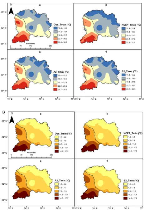
Fig. 5.(continued)
Table 7
AME and RMSSE between measured and predictedTmax,Tmin, and Precipitation for the period of 1991–2000, during kriging interpolation, in the Jhelum River basin.
Obs NCEP A2 B2
Tmin
AME (°C) 0.012 0.022 0.011 0.016
RMSSE 0.990 1.030 1.050 1.040
Tmax
AME(°C) 0.022 0.023 0.018 0.019
RMSSE 0.840 0.920 0.940 0.950
Precipitation
AME(°C) 7.300 11.600 7.200 7.900
RMSSE 1.150 1.100 1.200 1.160
Kriging method, using ArcGis 9.3.
3.4. Description of Kriging method
Kriging is an advanced, computationally intensive, geostatis-tical interpolation method (Buytaert et al., 2006) that takes care not only the distance but also the degree of variation among known data points when estimating values in unknown areas. The
first step in kriging interpolation is to inspect the data in order to identify the spatial structure, using empirical semivariogram or covariance. A semivariogram is a diagram that represents the connection between the distance (the distance between all the pairs of available data points) and semivariance, and covariance, in statistics, shows the strength of the correlation between two or more random variables. A basic principle on which the semivar-iogram bases is the points (stations, things etc.) closer to each other are more alike than the points that are farther apart.
The next step is to compute the weights for points from the model variogram. These weights are based on the distance be-tween the observed (measured) points and the prediction points, and also on the overall spatial relationships among the measured values surrounding the prediction location. In kriging, different statistical indicators such as Absolute Mean Error (AME), Root Mean Square Error (RMSE), Average Standard Error (ASE) and Root Mean Square Standardized Error (RMSSE) etc. and different graphs
such as graph between predicted and measured values, error graph and QQ-plot are used to check the performance of model (Pokhrel et al., 2013). Mathematical equations of these indicators are described in (Dai et al., 2014). In the present study, AME and RMSSE were used to check the performance of model. RMSSE is the ratio of RMSE to ASE. RMSSE and AME should be close to 1 and 0 respectively for satisfactory results. After satisfactory model performance, finally the maps were created for the study area. Mathematical detail about kriging method is described inPokhrel et al. (2013).
3.5. Future changes
After satisfactory calibration and validation, Tmax, Tmin, and P data was simulated for three spells—the 2020s (2011–2040), the 2050s (2041–2070), and the 2080s (2071–2099). The datasets of each of these periods were compared to a baseline period to analyze future changes in the basin. In this study, the period from 1961 to 1990 was taken as the baseline period because this period has been used in the majority of climate change studies across the world (Huang et al., 2011). A 30-year period is also considered long enough to define local climate because it is likely to include dry, wet, cool, and warm periods. The IPCC also recommends such a length (of 30 years) for the baseline period (Gebremeskel et al., 2005).
A
For better explanation, the temporal and spatial changes are presented graphically in this paper, as they have also been in other studies (Chu et al., 2010;Huang et al., 2011). Since Gulmarg and Qazigund weather stations lack data starting from 1961, the data for these stations was projected back by SDSM using NCEP predictors.
4. Results and discussion
4.1. Screening of predictors
Table 3 shows the predictors selected after screening, along with their mean absolute partial correlation (P.r) forTmax,Tmin, and Pat a significance level of 0.05. It was determined that tempera-ture at 2 m height (temp) was a super predictor for Tmax and Tmin in both the OPPB and TPPB sub-basins. A super predictor is the most prominent predictor and it displays maximum correlation with a predictand. For P, surface specific humidity (shum) and meridional wind velocity at 500 hPa (p5_v) were the most domi-nant predictors in the TPPB and OPPB respectively, for almost all weather stations. The selected predictors for P also expressed a logical sense because P depends mostly on water vapors (humid-ity) and wind direction. The selected predictors for the present study also match with the predictors used in several other studies
such asWilby et al. (2002),Chu et al. (2010),Huang et al. (2011), Hashmi et al. (2011), andMahmood and Babel (2012).
4.2. Calibration of SDSM
The explained variance (E), used as a performance indicator, ranged from 60% to 72% forTmax, 67% to 85% forTmin, and 8% to 32%
forP. The standard error (SE) forTmax,Tmin, andPwas 4.6°C, 3.4°C,
and 0.45 mm/day respectively. These results are satisfactory and comparable with the results of some previous studies likeWilby et al. (2002), Nguyen (2005), Liu et al. (2009), Souvignet and Heinrich (2011), andHuang et al. (2011). In this study, theEvalues forPwere much lower than theEvalues forTmaxandTmin. SinceP
is a heterogeneous climate variable and difficult to simulate, theE
ofPis more likely to be lower than 40%, while theEof temperature is more likely to be greater than 70% (Wilby et al., 2002).
4.3. Validation of SDSM
4.3.1. Tabular
For the validation of SDSM, three datasets were simulated by forcing the NCEP, A2, and B2 predictors, along with their calibrated parameters, for the period of 1991–2000, and for each of the local scale variables (Tmax,Tmin, andP). The performance indicators (R, R2, RMSE, and
m) were calculated using daily, monthly, and
B
seasonal time series from observed and simulatedTmax,Tmin, andP.
These are described inTables 4,5and6respectively. These tables show that the R2 values forT
max andTminwere
above 76%, 92% and 94% as calculated from daily, monthly, and seasonal time series respectively. TheR2values forPwere above 9%, 22%, and 50% as calculated from daily, monthly, and seasonal time series respectively. The results of Tmax and Tmin were better than the results of Pwith respect to all the indicators obtained from the daily, monthly, and seasonal time series, and Tmin results were slightly better than Tmax results. Although the R2 values obtained by the daily time series (ranging 8–15%) were much lower than those obtained by monthly (21–73%) and seasonal (25– 87%) time series when using NCEP predictors, these results are comparable with a previous study (Huang et al., 2011).
The main reason for lower values ofR2 for dailyPis the
oc-currence/amount of P, which is a stochastic process. Therefore, simulation ofPis always a difficult task (Huang et al., 2011). Sev-eral previous studies (Khan et al., 2006;Fealy and Sweeney, 2007; Huang et al., 2011) have shown worse results obtained from daily time series, compared to results obtained from monthly and sea-sonal time series. SDSM shows better applicability using monthly and seasonal P time series, relative to the daily time series. It was observed that the results obtained from NCEP predictors were better than A2 and B2 predictors, and the simulated data from A2 gave slightly better results than B2. Since SDSM is calibrated with
NCEP predictors, the calibrated parameters reflect some biases when the model is run with A2 and B2 predictors.
4.3.2. Graphical
The main purpose of graphical validation was to investigate the intra-annual variations in the TPPB, OPPB, and in the entire basin, as has been done in several studies (Wilby et al., 2002; Gebre-meskel et al., 2005;Zhao and Xu, 2008;Chu et al., 2010;Huang et al., 2011). For this, three datasets for Tmax, Tmin, and P were simulated by forcing the NCEP, A2, and B2 predictors into SDSM and the mean monthly, seasonal, and annual values were calcu-lated and compared with the observed datasets. However, in the present study, only P comparisons are shown graphically inFig. 4, which illustrates well the intra-annual variations in the TPPB, OPPB, and in the whole basin. The results ofTmaxandTminare not
shown graphically in the present study because the results ofTmax
andTmin(Tables 4and5) were quite satisfactory and much better
thanP. In addition,Pis a heterogeneous variable and it is difficult to capture its variations. Furthermore, it is the most important climate variable among all climate variables
Fig. 4(a) shows that in the TPPB, the big peak occurs in July– August (the monsoon season), and this was reasonably well si-mulated by all three datasets (NCEP, A2, and B2). On the other hand, the small peak, occurring in March, was underestimated by all three datasets. On the whole, the patterns were well followed by all three data sets.
C
The mean seasonal precipitations simulated from NCEP and A2 predictors were underestimated and overestimated by 7% and 6% respectively, except in spring (March–May). B2 showed under-estimations in winter (December–February) and spring and over-estimations in summer (June to August) and autumn (September– November). Overall, B2 underestimated with an average P of 0.89%. The mean annual precipitation from NCEP was under-estimated by 5.7% and from A2 and B2, it was overunder-estimated by 4% and 1.2% respectively.
Fig. 4(b) indicates that mean monthlyPwas not well simulated by SDSM in the OPPB as it was in the TPPB. Nonetheless, the patterns were followed by all three data sets. The NCEP, A2 and B2 datasets underestimated P in all seasons, with an average seasonal
Pof 6.9%, 11.8%, and 12% respectively, and an average annual P of 6.6%, 13% and 15% respectively.
Fig. 4(c) shows that the big peak was well simulated by all three data sets. However, the small peak was well underestimated by the model. The average seasonalP, as simulated by NCEP, A2 and B2, was underestimated by about 6.5%, 2.3% and 6.2% respectively. NCEP, A2, and B2 datasets underestimated the mean annualPby 6%, 3.45% and 5.75% respectively.
On the whole, SDSM performed reasonably well in capturing the variations of observed mean monthly, seasonal, and annualP. The results from NCEP dataset were better than A2 and B2 because the model was calibrated with NCEP dataset. Nonetheless, results from A2 and B2 datasets were quite comparable with NCEP. These results are also comparable with other studies (Chu et al., 2010; Huang et al., 2011)
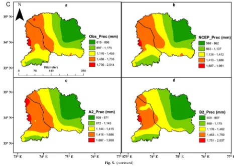
4.3.3. Spatial validation
To check the capability of SDSM in simulating spatial changes in the study area, three groups of maps (Fig. 5) for each variable (Tmax, Tmin, and P) were created by converting mean annual point data into raster data with the kriging interpolation method. As can be seen, each group has four maps; one was produced by using observed data and the other three by simulated data—one each from NCEP, A2 and B2 predictors. Two indicator, Absolute Mean Error (AME) and Root Mean Square Standardized Error (RMSSE) were utilized to check the performance of kriging method and results are described inTable 7. AME values forTmin,Tmaxand Pranged between 0.011°C and 0.022°C, 0.018°C and 0.23°C, and 7.2 mm and 11.6 mm respectively, in observed, NCEP, A2 and B2 maps, and RMSSE values forTmin,TmaxandPwere 0.99–1.05, 0.84–
0.95, and 1.1–1.2 respectively, which were quite satisfactory. It was seen that the spatial variations in observed mean annual temperature (TmaxandTmin) andPwere well reflected by all three
downscaled datasets, as is shown byFig. 5. Spatial distributions of temperature and precipitation showed that temperature decreases from south to north in accordance with the increase in elevation, andPdecreases from west to east. Spatial variability was reason-ably better simulated by NCEP data than by A2 and B2 data, and it was better captured in the TPPB than in the OPPB. Nevertheless, the results from A2 and B2 were comparable with NCEP.
Thus, it was concluded that SDSM is more credible in simulating mean monthly, seasonal and annual future changes in Tmax, Tmin, and P rather than in simulating daily future changes in the Jhelum basin. The calibrated SDSM, with NCEP predictors, can be used to
predict future changes inTmax,Tmin, andPbetter with respect to the
baseline period, than with A2 and B2 predictors.
5. Temporal and spatial future changes in temperature and precipitation
After successful calibration and validation, daily time series of
Tmax,Tmin, andPwere simulated for the 2020s, 2050s and 2080s
using A2 and B2 scenarios. Then, the calculated mean monthly, seasonal and annual Tmax,Tmin, and Pdata from the daily time
series was compared with the baseline data to analyze future changes in the 2020s, 2050s and 2080s (Chu et al., 2010;Huang et al., 2011).
5.1. Temporal changes
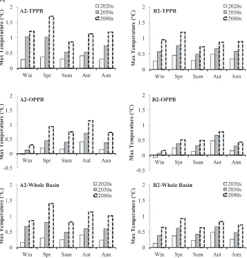
Fig. 6(A) shows mean annual and seasonal Tmax changes in the TPPB, OPPB, and in the whole Jhelum basin under A2 and B2 scenarios in the 2020s, 2050s and 2080s. Mean annualTmax, under
both scenarios, is projected to increase by 0.3–1.2°C in the TPPB, 0.14–0.74°C in the OPPB, and 0.24–1.02°C in the whole Jhelum basin in the 21st century.Kazmi et al. (2015)andRajbhandari et al. (2015) also showed increasing trends over the whole Pakistan. However, Kazmi et al. (2015)conducted study for the period of 2011–2013 and did not include the whole Jhelum basin because most of the Jhelum basin is situated in Jammu and Kashmir, and Rajbhandari et al. (2015)found out the projected changes over the Indus basin with Regional Climate Model. Similarly, all seasons show positive (increasing) changes under both scenarios in all three future periods (2020s, 2050s, and 2080s) except in winter in
the OPPB. Under A2 scenario, in the TPPB and OPPB, the most af-fected seasons are spring and autumn, with a projected increase of 1.7°C and 1.14°C in the 2080s respectively. In the whole basin, spring, with a 1.4°C increase in the 2080s, shows the most distinct change, relative to the other seasons. The same kinds of future changes are found under B2 but are relatively smaller in magni-tude than the changes under A2.
Fig. 6(B) illustrates the mean annual and seasonal changes in Tmin in the TPPB, OPPB, and in the whole basin under both sce-narios in the three future periods. Under both scesce-narios, mean annual Tmin is predicted to rise by 0.12–0.87°C in the TPPB, 0.03 to 0.31°C in the OPPB, and 0.04–0.65°C in the whole basin. These results are also supported byKazmi et al. (2015)andRajbhandari et al. (2015). In the case of seasonal changes, spring is affected more in the TPPB and autumn in the OPPB. The same is also the case ofTmax. Future changes inTminare predicted to be larger in
magnitude under A2 than B2, reflecting the same pattern for Tmax projections.
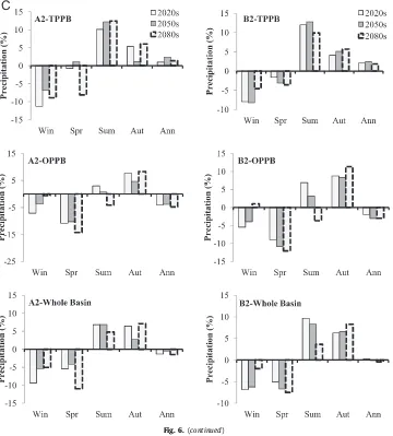
Fig. 6(C) presents the percentage changes in mean annual and seasonal P in the TPPB, OPPB, and in the whole basin under both scenarios. Mean annual P is estimated to increase by 1–3% in the TPPB and decrease by 2–5% in the OPPB, under both scenarios, with an overall decrease in the whole basin. As for seasonal changes in the TPPB basin, summer (the monsoon season in the basin) and autumn P show a definite increase of about 1–3% under A2 and 1–6% under B2 in the future, with the exception of the 2080s under B2. In contrast, in the TPPB, winter P is projected to decrease by 7–12% and 5–8% under A2 and B2, respectively. On the whole, in the TPPB, summer and autumn are more likely to receive increased P in the future with respect to the baseline values, and winter as well as spring are likely to receive less P in the future,
relative to the baseline values. These results are also supported by Rajbhandari et al. (2015). They conducted study for winter and summer monsoon and explored that summer precipitation is projected to increase and winter decrease.
In the OPPB, only autumn presents a definite increase inP(by 5–12%) in all three periods under both scenarios. In summer, the changes are positive in the 2020s and 2050s but negative in the 2080s.Pin spring (the peak season in the OPPB) is projected to decrease by 9–15% under both scenarios.
Therefore, it can be concluded that the peak in the OPPB is likely to go towards dryness in the future. In the whole basin, under both A2 and B2 scenarios, summer and autumn may be wetter than before, and winter and spring may be dryer, as com-pared to the baseline period. Since most of the meteorological
stations are installed in the valleys and not on the high altitudes (on Peaks) and the number of stations available inside the basin is insufficient, as shown in Fig. 1, temperature and precipitation changes in the basin might be different if the high altitudes will be considered.
5.2. Spatial changes
In this study, the mean annual changes inTmax,Tmin, andPwere
also analyzed spatially in the Jhelum River basin under A2 and B2 scenarios, with the help of kriging method, as shown inFig. 7. The AME and RMSSE between measured and predictedTmin,Tmax, and Pare presented inTable 8. AME ranged from 0.0002 to 0.09°C for Temperature (TmaxandTmin) and 0.34 to 1.2°C, respectively, and
RMSSE ranged from 0.74 to 1.004 for Temperature (TmaxandTmin)
and 0.92 to 1.005,respectively, under A2 and B2 in 2020s, 2050s and 2080s in the Jhelum River basin.
Fig. 7(A) shows the spatial distribution of mean annual chan-ges inTmaxin the 2020s, 2050s and 2080s under A2 and B2
sce-narios, relative to the baseline. The northwest part of the basin is projected to be the most affected in all three future periods, with a definite increase inTmax. The southeast part of the basin is
pre-dicted to be the least affected.Tmaxonly shows a small increase in
this region. The results also indicate that the changes are mostly increasing moving from southeast to northwest side under both scenarios.
Fig. 7 (B) presents the spatial distribution of mean annual changes inTminin the three future periods under A2 and B2
sce-narios, relative to the baseline. Most of the basin shows decrease in Tmin under A2 in 2020s and 2050s and most of the basin
Table 8
AME and RMSSE between predicted Tmax, Tmin, and Precipitation for the period of 2020s, 2050s and 2080s, during kriging interpolation, in the Jhelum River basin.
2020s 2050s 2080s
Tmin A2 B2 A2 B2 A2 B2
AME (°C) 0.0300 0.0100 0.0900 0.0500 0.0120 0.0800 RMSSE 0.9000 0.8611 0.9155 0.9259 0.8750 0.7595 Tmax
AME(°C) 0.0200 0.0200 0.0002 0.0200 0.0056 0.0240 RMSSE 1.0043 1.0909 0.9211 0.9333 0.9574 0.9189
Precipitation
AME(°C) 0.6100 0.4300 0.4500 0.3400 1.2000 0.7800 RMSSE 0.9281 0.9455 0.9400 0.9180 1.0047 0.9644
AME¼Absolute Mean Error,RMSSE¼Root Mean Square Standardized Error
presents increase in 2080s. Under B2, almost half of the basin gives indication about decrease inTminin 2020s. However, most of the
basin shows increaseTminin 2050s and 2080s.
Fig. 7(C) provides the spatial distribution of percentage chan-ges in mean annualP, as compared to the baseline under A2 and B2 scenarios in all three future periods. As can be seen, on the whole, the changes are spread between 13% and 16% over the whole basin under both scenarios, in all three future periods. The simulated decrease in P occurs in eastern part and increases in the west of the basin. It can be seen that almost half of the basin shows decreasing P in the 2020s. However, in the 2080s, it is projected that more than half of the basin will have decreasedP
under both scenarios. Under both scenarios, similar kinds of spa-tial distribution patterns of mean annual precipitation changes can be seen, for all three future periods; however, the changes (posi-tive or nega(posi-tive) are higher under A2 than under B2.
6. Conclusions
In this study, a well-known decision support tool, the Statistical Downscaling Model (SDSM), was applied to analyze the temporal and spatial future changes in maximum temperature, minimum temperature and precipitation in the sub-basins, TPPB and OPPB, and in the whole Upper Jhelum River basin under A2 and B2 scenarios. The downscaling of these variables is very important in order to study the impacts of climate change on the hydrological cycle of the basin.
SDSM showed good capability in simulating Tmax and Tmin in daily, monthly, and seasonal time series, during the calibration and validation. However, it presented good results only for monthly and seasonal precipitation. However, only seasonal and annual future changes, with respect to baseline, were presented in this study. Seasonal data was simulated better than monthly and daily data.
Mean annual Tmax and Tmin were projected to increase in both parts of the Jhelum basin, the TPPB and the OPPB, under both scenarios, and in all three future periods. This simulated increase in temperature was higher under A2 than B2 in both the sub-ba-sins and it was higher in the TPPB than OPPB. For seasonal changes in mean annual temperature (Tmax and Tmin), the maximum increase was projected for spring under both scenarios (A2 and B2) in the whole basin. Spring in the TPPB and autumn in the OPPB were projected to be the most affected seasons as far as rise in temperature was concerned.
Mean annual precipitation was predicted to increase by 1–3% in the TPPB and decrease by 2–5% in the OPPB under both scenarios, with an overall decrease in the whole basin. Summer and winter were the most affected seasons in the TPPB under both scenarios and in all three future periods. In the OPPB, autumn showed in-crease in precipitation, and spring showed dein-crease under both scenarios. As for the whole basin, summer and autumn were projected to receive more precipitation, and winter as well as spring to receive lesser amounts of precipitation in the future, as compared to baseline period.
The spatial distribution of mean annualTmaxshowed a rise in
almost all parts of the basin in the future periods, relative to the baseline period. However, northwestern parts of the basin were projected to face a higher increase than southeastern parts under both scenarios.Tminwas projected to decrease in some parts of the
basin but a majority of the basin will experience a rise in Tmin
under both scenarios especially in 2050s and 2080s, as compared to the baseline values. It was seen that almost half of the basin showed decreasing precipitation in the 2020s, but in the 2080s, decreasing precipitation was likely to be experienced in most parts of the basin under both scenarios. Both scenarios presented similar
kinds of spatial distribution patterns of mean annual Tmax, Tmin, and precipitation changes in all three future periods, but with different magnitudes. The changes under A2 were observed higher than under B2.
Acknowledgments
This study is a part of thefirst author’s doctoral research work, conducted at the Asian Institute of Technology Thailand. The au-thors wish to acknowledge and offer gratitude to Pakistan Me-teorological Department (PMD), the Water and Power Develop-ment Authority (WAPDA) of Pakistan, the India Meteorological Department (IMD), and the National Climate Data Center (NCDC), for providing important and valuable data for the research. Heartfelt gratitude is also extended to the Higher Education Commission (HEC) of Pakistan and AIT for providing financial support to thefirst author for his doctoral studies at AIT.
References
Ahmad, I., Ambreen, R., Sun, Z., Deng, W., 2015. Winter-Spring Precipitation Variability in Pakistan. Am. J. Clim. Change 4 (1), 115–139.http://dx.doi.org/ 10.4236/ajcc.2015.41010.
Ahmad, N., Chaudhry, G.R., 1988. Irrigated agriculture of Pakistan S. Nazir, Lahore. Akhtar, M., Ahmad, N., Booij, M.J., 2008. The impact of climate change on the water resources of Hindukush–Karakorum–Himalaya region under different glacier coverage scenarios. J. Hydrol. 355 (1-4), 148–163.http://dx.doi.org/10.1016/j. jhydrol.2008.03.015.
Akhtar, M., Ahmad, N., Booij, M.J., 2009. Use of regional climate model simulations as input for hydrological models for the Hindukush-Karakorum-Himalaya re-gion. Hydrol. Earth Syst. Sci. 13 (7), 1075–1089.http://dx.doi.org/10.5194/ hess-13-1075-2009.
Anandhi, A., Srinivas, V.V., Nanjundiah, R.S., Nagesh Kumar, D., 2007. Downscaling precipitation to river basin in India for IPCC SRES scenarios using support vector machine. Int. J. Climatol. 28, 401–420.http://dx.doi.org/10.1002/joc.1529. Archer, D.R., Fowler, H.J., 2008. Using meteorological data to forecast seasonal
runoff on the River Jhelum, Pakistan. J. Hydrol. 361 (1-2), 10–23.http://dx.doi. org/10.1016/j.jhydrol.2008.07.017.
Ashiq, M., Zhao, C., Ni, J., Akhtar, M., 2010. GIS-based high-resolution spatial in-terpolation of precipitation in mountain–plain areas of Upper Pakistan for re-gional climate change impact studies. Theor. Appl. Climatol. 99 (3), 239–253. http://dx.doi.org/10.1007/s00704-009-0140-y.. http://dx.doi.org/10.1007/ s00704-009-0140-y.
Benestad, R.E., Hansen-Bauer, I., Chen, D., 2008. Empirical-statistical Downscaling. World Scientific, New York, p. 215.
Buytaert, W., Celleri, R., Willems, P., Bièvre, B.D., Wyseure, G., 2006. Spatial and temporal rainfall variability in mountainous areas: a case study from the South Ecuadorian Andes. J. Hydrol. 329 (3–4), 413–421.http://dx.doi.org/10.1016/j. jhydrol.2006.02.031.
CCCSN, 2012. Statistical Downscaling Input: HadCM3 Predictors: A2 and B2 Experiments.
Chu, J., Xia, J., Xu, C.Y., Singh, V., 2010. Statistical downscaling of daily mean tem-perature, pan evaporation and precipitation for climate change scenarios in Haihe River, China. Theor. Appl. Climatol. 99 (1), 149–161.http://dx.doi.org/ 10.1007/s00704-009-0129-6.
Dai, F., Zhou, Q., Lv, Z., Wang, X., Liu, G., 2014. Spatial prediction of soil organic matter content integrating artificial neural network and ordinary kriging in Tibetan Plateau. Ecol. Indic. 45 (0), 184–194.http://dx.doi.org/10.1016/j. ecolind.2014.04.003.
Diaz-Nieto, J., Wilby, R.L., 2005. A comparison of statistical downscaling and climate change factor methods: impacts on lowflows in the River Thames, United Kingdom. Clim. Change 69 (2), 245–268.http://dx.doi.org/10.1007/s10584-005-1157-6. Fealy, R., Sweeney, J., 2007. Statistical downscaling of precipitation for a selection of
sites in Ireland employing a generalised linear modelling approach. Int. J. Cli-matol. 27 (15), 2083–2094.http://dx.doi.org/10.1002/joc.1506.
Fowler, H.J., Blenkinsop, S., Tebaldi, C., 2007. Linking climate change modelling to impacts studies: recent advances in downscaling techniques for hydrological modelling. Int. J. Climatol. 27 (12), 1547–1578.http://dx.doi.org/10.1002/ joc.1556.
Gagnon, S., Singh, B., Rousselle, J., Roy, L., 2005. An application of the statistical downscaling model (SDSM) to simulate climatic data for streamflow modelling in Québec, Canada. Water Resour. J. 30 (4), 297–314.http://dx.doi.org/10.4296/ cwrj3004297.
Ghosh, S., Mujumdar, P., 2008. Statistical downscaling of GCM simulations to streamflow using relevance vector machine. Water Resour. 31, 132–146. Goyal, M.K., Ojha, C.S.P., 2010. Robust weighted regression as a downscaling tool in
temperature projections. Int. J. Glob. Warm. 2 (3), 234–251.http://dx.doi.org/ 10.1504/IJGW.2010.036135.
Hashmi, M.Z., Shamseldin, A.Y., Melville, B.W., 2011. Comparison of SDSM and LARS-WG for simulation and downscaling of extreme precipitation events in a watershed. Stoch. Env. Res. Risk A 25 (4), 475–484.http://dx.doi.org/10.1007/ s00477-010-0416-x.
Hay, L.E., Clark, M.P., 2003. Use of statistically and dynamically downscaled atmo-spheric model output for hydrologic simulations in three mountainous basins in the western United States. J. Hydrol. 282 (1–4), 56–75.http://dx.doi.org/ 10.1016/s0022-1694(03)00252-x.
Hay, L.E., Wilby, R.L., Leavesley, G.H., 2000. A comparison of delta change and downscaled GCM scenarios for three mountainous basins in the United States. J. American Water Resour. Ass. 36 (2), 387–397.http://dx.doi.org/10.1111/ j.1752-1688.2000.tb04276.x.
Huang, J., et al., 2011. Estimation of future precipitation change in the Yangtze River basin by using statistical downscaling method. Stoch. Env. Res. Risk A. 25 (6), 781–792.http://dx.doi.org/10.1007/s00477-010-0441-9.
IPCC, 2013. Climate Change 2013: The Physical Science Basis. Contribution of Working Group I to the Fifth Assessment Report of the Intergovern–Mental Panel on Climate Change Cambridge University Press, Cambridge, United Kingdom and New York, NY, USA.
Jacobusse, G., 2005. WinMICE User’s manual.
Kazmi, D., et al., 2015. Statistical downscaling and future scenario generation of temperatures for Pakistan Region. Theor. Appl. Climatol. 120 (1–2), 341–350. http://dx.doi.org/10.1007/s00704-014-1176-1.
Khan, M.S., Coulibaly, P., Dibike, Y., 2006. Uncertainty analysis of statistical down-scaling methods. J. Hydrol. 319 (1-4), 357–382.http://dx.doi.org/10.1016/j. jhydrol.2005.06.035.
Liu, J., Williams, J.R., Wang, X., Yang, H., 2009. Using MODAWEC to generate daily weather data for the EPIC model. Environ. Model. Softw. 24 (5), 655–664.http: //dx.doi.org/10.1016/j.envsoft.2008.10.008.
Mahmood, R., Babel, M., 2012. Evaluation of SDSM developed by annual and monthly sub-models for downscaling temperature and precipitation in the Jhelum basin, Pakistan and India. Theor. Appl. Climatol., 1–18.http://dx.doi.org/ 10.1007/s00704-012-0765-0.
Mujumdar, P., Ghosh, S., P., 2008. Modeling GCM and scenario uncertainty using a possibilistic approach: application to the Mahanadi River, India. Water Resour. Res. 44, W06407-1.
Nguyen, V., 2005. Downscaling methods for evaluating the impacts of climate change and variability on hydrological regime at basin scale. In: Proceedings of the International Symposium on Role of Water Sciences in Transboundary River Basin Management, Thailand, pp. 1–8.
Opitz-Stapleton, S., Gangopadhyay, S., 2010. A non-parametric, statistical
downscaling algorithm applied to the Rohini River Basin, Nepal. Theor. Appl. Climatol. 103 (3–4), 375–386.http://dx.doi.org/10.1007/s00704-010-0301-z. Pokhrel, R.M., Kuwano, J., Tachibana, S., 2013. A kriging method of interpolation
used to map liquefaction potential over alluvial ground. Eng. Geology. 152 (1), 26–37.http://dx.doi.org/10.1016/j.enggeo.2012.10.003.
Qamer, F.M., Saleem, R., Hussain, N., Raza, S.M., 2008. Multi-scale watershed da-tabase of Pakistan. In: Proceedings of the 10th International Symposium on High Mountain Remote Sensing Cartography.
Rajbhandari, R., Shrestha, A.B., Kulkarni, A., Patwardhan, S.K., Bajracharya, S.R., 2015. Projected changes in climate over the Indus river basin using a high re-solution regional climate model (PRECIS). Clim Dyn. 44 (1-2), 339–357.http: //dx.doi.org/10.1007/s00382-014-2183-8.
Souvignet, M., Heinrich, J., 2011. Statistical downscaling in the arid central Andes: uncertainty analysis of multi-model simulated temperature and precipitation. Theor. Appl. Climatol. 106 (1-2), 229–244.http://dx.doi.org/10.1007/ s00704-011-0430-z.
Tripathi, S., Srinivas, V.V., Nanjundiah, R.S., 2006. Downscaling of precipitation for climate change scenarios: a support vector machine approach. J. Hydrol. 330 (3–4), 621–640.http://dx.doi.org/10.1016/j.jhydrol.2006.04.030.
Wetterhall, F., Bárdossy, A., Chen, D., S.H., C.-Y, X., 2006. Daily precipitation-downscaling techniques in three Chinese regions. Water Resour. Res. 42, W11423.http://dx.doi.org/10.1029/2005WR004573.
Wilby, R.L., Dawson, C.W., Barrow, E.M., 2002. SDSM—a decision support tool for the assessment of regional climate change impacts. Environ. Model. Softw. 17 (2), 145–157.http://dx.doi.org/10.1016/s1364-8152(01)00060-3.
Wilby, R.L., et al., 2000. Hydrological responses to dynamically and statistically downscaled climate model output. Geophys. Res. Lett. 27 (8), 1199.http://dx. doi.org/10.1029/1999GL006078.
Wilby, R.L., Hay, L.E., Leavesley, G.H., 1999. A comparison of downscaled and raw GCM output: implications for climate change scenarios in the San Juan River basin, Colorado. J. Hydrol. 225 (1–2), 67–91.http://dx.doi.org/10.1016/ s0022-1694(99)00136-5.
Wilby, R.L., et al., 2006. Integrated modelling of climate change impacts on water resources and quality in a lowland catchment: River Kennet, UK. J. Hydrol. 330 (1–2), 204–220.http://dx.doi.org/10.1016/j.jhydrol.2006.04.033.
Xu, C.Y., 1999. Climate change and hydrologic models: a review of existing gaps and recent research developments. Water Resour. Manag. 13 (5), 369–382.http: //dx.doi.org/10.1023/a:1008190900459.
Zhang, X.C., Liu, W.Z., Li, Z., Chen, J., 2011. Trend and uncertainty analysis of si-mulated climate change impacts with multiple GCMs and emission scenarios. Agric. For. Meteorol. 151 (10), 1297–1304.http://dx.doi.org/10.1016/j. agrformet.2011.05.010.