Power Kites for Wind Energy Generation
Fast Predictive Control of Tethered Airfoils
BY MASSIMO CANALE, LORENZO FAGIANO, and MARIO MILANESE
T
he problems posed by electric energy generation from fossil sources include high costs due to large demand and limited resources, pollution and CO2production,and the geopolitics of producer countries. These problems can be overcome by alternative sources that are renewable, cheap, easily available, and sustainable. However, current renewable technologies have limitations. Indeed, even the most optimistic forecast on the diffusion of wind, photo-voltaic, and biomass sources estimates no more than a 20%
contribution to total energy production within the next 15–20 years.
Excluding hydropower plants, wind turbines are cur-rently the largest source of renewable energy [1]. Unfortu-nately, wind turbines require heavy towers, foundations, and huge blades, which impact the environment in terms of land usage and noise generated by blade rotation, and require massive investments with long-term amortization. Consequently, electric energy production costs are not yet competitive with thermal generators, despite recent increases in oil and gas prices.
THE KITEGEN PROJECT
To overcome the limitations of current wind power tech-nology, the KiteGen project was initiated at Politecnico di Torino to design and build a new class of wind energy generators in collaboration with Sequoia Automation, Modelway, and Centro Studi Industriali. The project focus [2], [3] is to capture wind energy by means of controlled tethered airfoils, that is, kites; see Figure 1.
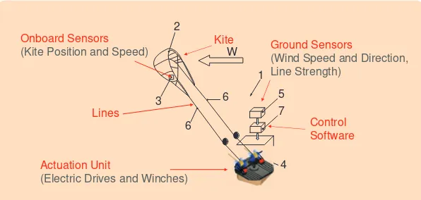
The KiteGen project has designed and simulated a small-scale prototype (see Figure 2). The two kite lines are rolled around two drums and linked to two electric drives, which are fixed to the ground. The flight of the kite is con-trolled by regulating the pulling force on each line. Energy is collected when the wind force on the kite unrolls the lines, and the electric drives act as generators due to the rotation of the drums. When the maximal line length of about 300 m is reached, the drives act as motors to recover the kite, spending a small percentage (about 12%, see the “Simulation Results” section for details) of the previously
generated energy [4]. This yo-yo configurationis under the control of the kite steering unit (KSU, see Figure 3), which includes the electric drives (for a total power of 40 kW), the drums, and all of the hardware needed to control a single kite. The aims of the prototype are to demonstrate the abil-ity to control the flight of a single kite, to produce a signifi-cant amount of energy, and to verify the energy production levels predicted in simulation studies.
The potential of a similar yo-yo configuration is investi-gated, by means of simulation results, in [5] and [6] for one or more kites linked to a single cable. In [5] and [6], it is assumed that the angle of incidence of the kites can be controlled. Thus, the control inputs are not only the roll angle ψand the cable winding speed, as considered in [4] and in this article, but also the lift coefficient CL.
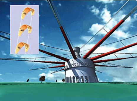
For medium-to-large-scale energy generators, an alter-native KiteGen configuration is being studied, namely, the
carousel configuration. In this configuration, introduced in [7] and shown in Figure 4, several airfoils are controlled by their KSUs placed on the arms of a verti-cal-axis rotor. The controller of each kite is designed to maximize the torque exerted on the rotor, which transmits its motion to an electric generator. For a given wind direction, each airfoil can produce energy for about 300◦ of carousel rotation; only a small fraction (about 1%, see the “Simula-tion Results” sec“Simula-tion for details) of the generated energy is used to drag the kite against the wind for the remaining 60◦.
According to our simulation results, it is estimated that the required land usage for a kite generator may be lower than a current wind farm of the same power by a factor of up to 30–50, with electric energy FIGURE 1 Kite surfing. Expert kite-surfers drive kites to obtain
ener-gy for propulsion. Control technoloener-gy can be applied to exploit this technique for electric energy generation.
FIGURE 2 KiteGen small-scale prototype of a yo-yo configuration. The kite lines are linked to two electric drives. The flight of the kite is controlled by regulating the pulling force on each line, and energy is generated as the kite unrolls the lines.
FIGURE 3 Scheme of the kite steering unit. The kite steering unit, which provides auto-matic control for KiteGen, includes the electric drives, drums, and all of the hardware needed to control a single kite.
Onboard Sensors
(Kite Position and Speed)
Lines
Actuation Unit
(Electric Drives and Winches)
Kite W
1
6 5
7 6
3
4 2
Control Software Ground Sensors
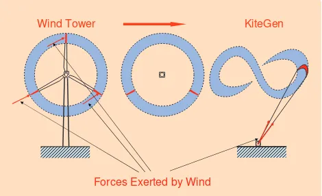
production costs lower by a factor up to 10–20. Such poten-tial improvement over current wind technology is due to several aerodynamic and mechanical reasons [8], [9]. For example, 90% of the power generated by a 2-MW three-blade turbine with a 90-m rotor diameter is contributed by only the outer 40% of the blade area, corresponding to about 120 m2. This dependence is due to the fact that the aerodynamic forces on each infinitesimal section of the blades are proportional to the square of its speed with respect to the air, and this speed increases toward the tip of the blades. In KiteGen, the tethered airfoils act as the outer portions of the blades, without the need for mechanical support of the tower and of the less-productive inner blade portions; see Figure 5. Indeed, a mean generated power of 620 kW is obtained in the simulation reported in Figure 16 for a single kite of 100-m2area and 300-m line length.
Figure 5 shows that the torque exerted by wind forces at the base of a wind turbine’s support structure increases with
FIGURE 4 KiteGen carousel configuration concept. Several airfoils are controlled by the kite steering units placed on the arms of a ver-tical axis rotor. The airfoils’ flight is controlled so as to turn the rotor, which transmits its motion to an electric generator.
A
t present, a small scale yo-yo prototype has been real-ized (see Figure S1). This system can generate up to 40 kW using commercial kites with characteristic area up to 10 m2and line length up to 800 m. The prototype is under test (see Figure S2). Preliminary tests show that the amount of energy predicted by simulation is confirmed by experimental data.A new KiteGen prototype is expected to be built in the next 24–36 months to demonstrate the energy-generation capabilities of the carousel configuration. In particular, a carousel structure with a single kite steering unit mounted
on a cart riding on a circular rail will be considered. To col-lect the energy produced by the wagon motion, the wheels of the cart are connected to an alternator. Such a proto-type is expected to produce about 0.5 MW with a rail radius of about 300 m. According to scalability, a platoon of carts, each one equipped with a kite steering unit, can be mounted on the rail to obtain a more effective wind power plant. This configuration can generate, on the basis of preliminary computations, about 100 MW at a produc-tion cost of about 20 €/MWh, which is two to three times lower than from fossil sources.
FIGURE S1 The first KiteGen prototype. Based on the yo-yo con-figuration, KiteGen can generate up to 40 kW using commercial kites with characteristic area up to 10 m2and line length up to 800 m. Preliminary tests show that the amount of energy predict-ed by simulation is confirmpredict-ed by experimental data. A new Kite-Gen prototype is expected to be built in the next 24 to 36 months to demonstrate energy-generation capabilities of the carousel configuration.
FIGURE S2 KiteGen small scale prototype flying tests. This pic-ture shows the kite motion and line developing during the trac-tion phase. The kite steering unit is mounted on a light truck for easy transportation to locations with favorable wind conditions. This picture was taken on a hill near Torino.
the height of the tower, the force is independent of the line length in KiteGen. Due to structural and economical limits, it is not convenient to go beyond the 100–120 m height of the largest turbines commercially available. In contrast, airfoils can fly at altitudes up to several hundred meters, taking advantage of the fact that, as altitude over the ground increas-es, the wind is faster and less variable; see Figure 6. For exam-ple, at 800 m the mean wind speed doubles with respect to 100 m (the altitude at which the largest wind turbines operate). Since the power that can be extracted from wind grows with the cube of the wind speed, the possibility of reaching such heights represents a further significant advantage of KiteGen.
The carousel configuration is scalable up to several hundred megawatts, leading to increasing advantages over current wind farms. Using data from the Danish
Wind Industry Association Web site [10], it follows that, for a site such as Brindisi, in the south of Italy, a 2-MW wind turbine has a mean production of 4000 MWh/year. To attain a mean generation of 9 TWh/year, which corre-sponds to almost 1000-MW mean power, 2250 such towers are required, with a land usage of 300 km2and an energy production cost of about 100–120 €/MWh. In comparison, the production cost from fossil sources (gas, oil) is about 60–70 €/MWh. Simulation results show that a KiteGen capable of generating the same mean energy can be realized using 60–70 airfoils of about 500 m2, rotating in a carousel configuration of 1500-m radius and flying up to 800 m. The resulting land usage is 8 km2, and the energy production cost is estimated to be about 10–15 €/MWh.
SYSTEM AND CONTROL TECHNOLOGIES
NEEDED FOR KITEGEN
Control Design
The main objective of KiteGen control is to maximize energy generation while preventing the airfoils from falling to the ground or the lines from tangling. The control problem can be expressed in terms of maximizing a cost function that pre-dicts the net energy generation while satisfying constraints on the input and state variables. Nonlinear model predictive control (MPC) [11] is employed to accomplish these objec-tives, since it aims to optimize a given cost function and fulfill constraints at the same time. However, fast implementation is needed to allow real-time control at the required sampling time, which is on the order of 0.1 s. In particular, the imple-mentation of fast model predictive control (FMPC) based on set membership approximation methodologies as in [12] and [13] is adopted, see “How Does FMPC Work ?” for details.
Model Identification
Optimizing performance for Kite-Gen relies on predicting the behav-ior of the system dynamics as accurately as possible. However, since accurately modeling the dynamics of a nonrigid airfoil is challenging, model-based control design may not perform satisfacto-rily on the real system. In this case, methods for identifying nonlinear systems [14], [15] can be applied to derive more accurate models.
Sensors and Sensor Fusion
The KiteGen controller is based on feedback of the kite position and speed vector, which must be mea-sured or accurately estimated. Each airfoil is thus equipped with a pair of triaxial accelerometers and a pair FIGURE 5 Comparison between wind turbines and airfoils in energy
production. In wind towers, limited blade portions (red) contribute predominantly to power production. In KiteGen, the kite acts as the most active portions of the blades, without the need for mechanical support of the less active portions and the tower.
Forces Exerted by Wind
Wind Tower KiteGen
FIGURE 6 Wind-speed variation as a function of altitude. These data are based on the average European wind speed of 3 m/s at ground level. Source: Delft University, Dr. Wubbo Ockels.
Altitude (m)
3,000 2,800 2,600 2,400 2,200 2,000 1,800 1,600 1,400 1,200 1,000 800 600 400 200 0
Wind Speed (m/s)
T
he fast model predictive control (FMPC) approach intro-duced and described in [12] and [13] is based on set mem-bership techniques. The main idea is to find a function fˆthat approximates the exact predictive control law ψ(tk)= f(w(tk))to a specified accuracy. Evaluating the approximating function is faster than solving the constrained optimization problem con-sidered in MPC design.
To be more specific, consider a bounded region W⊂R8 where wcan evolve. The region Wcan be sampled by choosing
˜
wk∈W, k=1, . . . , ν, and computing offline the corresponding exact MPC control given by
˜
ψk= f(wk˜ ), k=1, . . . , ν. (S1)
The aim is to derive, from these known values of ψ˜k and wk˜ and from known properties of f, an approximation fˆof f over
W, along with a measure of the approximation error. Neural networks are used in [S1] for such an approximation. However, neural networks have limitations, such as the possibility of local minima during the learning phase and the difficulty of sat-isfying the constraints in the image set of the function to be approximated. Moreover, no measure of the approximation error is provided. To overcome these drawbacks, a set mem-bership approach is used in [12] for MPC with linear models. Based on sampled data and a priori information about f, the approach finds a feasible function set in which the true function is guaranteed to lie. An optimal approximation, along with approximation error, is derived based on this set. In the case of KiteGen control it is assumed that f ∈Fγ, where Fγ is the set
of Lipschitz functions on Wwith Lipschitz constant γ. Note that stronger assumptions cannot be made, since even in the sim-ple case of linear dynamics and a quadratic functional, f is a piecewise linear continuous function [S2]. In addition, the input saturation condition gives the a priori bound |f(w)| ≤ ¯ψ. This information about the function f, combined with the values of the function at the points wk˜ ∈W, k=1, . . . , ν, implies that f
is a member of the feasible function set
F F S= {f∈Fγ :|f(w)| ≤ ¯ψ;f(wk˜ )= ˜ψk, k=1, . . . , ν}, (S2)
which summarizes the available information on f. Set membership theory facilitates the derivation of an optimal estimate of f and its approximation error in terms of the Lp(W) norm for p∈[1,∞],
of points, the error between fˆand f is unknown. However, given the a priori information, the tightest guaranteed bound is given by
A function f∗is optimal approximationif
rp=. E(f∗)=inf
ˆ
f E(f),
where the radius of information rpgives the minimal Lp approxima-tion error that can be guaranteed. Defining
f(w)=. min
which is an optimal approximation in the Lp(W) norm for all
p∈[1,∞] [13]. Moreover, the approximation error of f∗is point-wise bounded as
|f(w)−f∗(w)| ≤1
2|f(w)−f(w)|,for allw∈W
and is pointwise convergent to zero [13]
lim
tation of ψ˜k are sufficient to achieve a desired accuracy in the estimation of f or if the value of νmust be increased. Then, the MPC control can be approximately implemented online by evalu-ating the function f∗(wt
k)at each sampling time so that
ψtk= f ∗(wt
k).
As νincreases, the approximation error decreases at the cost of increased computation time.
REFERENCES
[S1] T. Parisini and R. Zoppoli, “A receding-horizon regulator for nonlinear systems and a neural approximation,” Automatica, vol. 31, no. 10, pp. 1443–1451, 1995.
[S2] A. Bemporad, M. Morari, V. Dua, and E.N. Pistikopoulos “The explicit linear quadratic regulator for constrained systems,” Auto-matica,vol. 38, pp. 3–20, 2002
of triaxial magnetometers placed at the airfoil’s extreme edges, which transmit data to the control unit by means of radio signals. These data are sufficient for estimating the kite position and speed. However, in order to improve esti-mation accuracy and to achieve some degree of recovery in the case of sensor failure, we plan to use a load cell to mea-sure the length and traction force of each line as well as a vision system to determine the kite angular position.
A key issue in KiteGen operation is the detection and recovery of possible breakdowns or malfunctions of the sensors. For example, the vision system may not operate in the presence of clouds, haze, or heavy rain. A common way to treat this problem is to use estimation techniques based on the system model and available measurements. However, due to the kite’s nonlinear dynamics, the extended Kalman filter (EKF), based on approximations of the nonlinearities, gives rise to numerical stability prob-lems and severe accuracy deterioration. Moreover, the EKF design is based on a model that, although quite complex and nonlinear, is only an approximate description of the actual system. Alternatively, the direct virtual sensor (DVS) approach [16], [17] facilitates the design of an opti-mal filter based on experimental data collected in the absence of sensor faults. In particular, when an accurate model is available and the noise statistical hypotheses are
fulfilled, the DVS gives the same accuracy as the theoreti-cal minimal variance filter. Moreover, in the presence of modeling errors and nonlinearities, the DVS guarantees stability and performs tradeoffs between optimality and robustness, which are not achievable with EKF.
KITE GENERATOR MODELS
Kite Dynamics
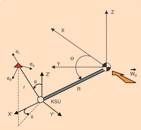
The model developed in [18] describes the kite dynamics. A fixed cartesian coordinate system (X,Y,Z)is considered (see Figure 7), with the Xaxis aligned with the nominal wind speed vector. The wind speed vector is represented as Wl= W0+ Wt, where W0is the nominal wind, assumed
where Wx(Z) is a known function that gives the wind
nominal speed at each altitude Z(see Figure 6). The term
Wtmay have components in all directions and is assumed
to be unknown, accounting for unmeasured turbulence. A second cartesian coordinate system (X′,Y′,Z′), cen-tered at the KSU location, is introduced to take into account possible KSU motion with respect to (X,Y,Z); oth-erwise, (X′,Y′,Z′)≡(X,Y,Z) is assumed. In this system, the kite position can be expressed as a function of its dis-tance rfrom the origin and the angles θand φ, as depicted in Figure 7, which also shows the basis vectors eθ, eφ, erof
a local coordinate system centered at the kite location. Applying Newton’s laws of motion to the kite in the local coordinate system yields
¨
include the contributions of the gravitational force mg, apparent force Fapp , aerodynamic force Faer , and the force
Fc exerted by the lines on the kite. Expressed in the local
coordinates, the forces are given by
Fθ=(sinθ )mg+Fapp,θ+Faer,θ, (5)
Fφ=Fapp,φ+Faer,φ, (6)
Fr= −(cosθ )mg+Fapp,r+Faer,r−Fc. (7)
Apparent Forces
The components of the apparent force vector Fapp depend on the kite generator configuration. For example, for the yo-yo FIGURE 7 Model of a single kite steering unit. A fixed cartesian
coor-dinate system (X,Y,Z)is considered, with the Xaxis aligned with the direction of the nominal wind speed vector W0. A second carte-sian coordinate system (X′,Y′,Z′), centered at the KSU location, is considered when KSU is moving with respect to (X,Y,Z). In the yo-yo configuration, since the KSU location is fixed at the ground,
(X′,Y′,Z′)≡(X,Y,Z) is assumed. In the coordinate system
(X′,Y′,Z′), the kite position can be expressed as a function of its distance r from the origin and of the two angles θ and φ. In the carousel configuration, the KSU rotates around the origin of
configuration, centrifugal inertial forces have to be considered, that is, Fapp = Fapp(θ, φ,r,θ ,˙ φ,˙ ˙r). For the carousel configura-tion, since each KSU moves along a circular trajectory with constant radius R(see Figure 7), the carousel rotation angle and its derivatives must be included in the apparent force cal-culation, so that Fapp= Fapp(θ, φ,r, ,θ ,˙ φ,˙ ˙r,,˙ )¨ .
Aerodynamic Forces
The aerodynamic force Faer depends on the effective wind speed We, which in the local system is computed as
We= Wa− Wl, (8)
where Wais the kite speed with respect to the ground. For
both the yo-yo and carousel configurations, Wa can be
expressed as a function of the local coordinate system (φ, θ,r) and the position of the KSU with respect to the fixed coordinate system (X,Y,Z).
Let us consider now the kite wind coordinate system, with its origin located at the kite center of gravity, the basis vector xwaligned with the effective wind speed vector, the basis vector zwcontained by the kite longitudinal plane of symmetry and pointing from the top surface of the kite to the bottom, and the basis vector yw completing a right-handed system. In the wind coordinate system the aerody-namic force Faer,w is given by
Faer,w=FDxw +FLzw, (9)
where FDis the drag force and FLis the lift force,
comput-ed as
FD= −1
2CDAρ|We|
2, (10)
FL= −1
2CLAρ|We|
2, (11)
where ρis the air density, Ais the kite characteristic area, and CLand CDare the kite lift and drag coefficients. All of
these variables are assumed to be constant. The aerody-namic force Faer can then be expressed in the local coordi-nate system as a nonlinear function of several arguments of the form
Faer= ⎛
⎝
Faer,θ(θ, φ,r, ψ,We)
Faer,φ(θ, φ,r, ψ,We)
Faer,r(θ, φ,r, ψ,We) ⎞
⎠. (12)
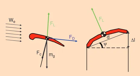
The kite roll angle ψin (12) is the control variable, defined by
ψ=arcsin
l d
, (13)
where dis the kite width and lis the length difference between the two lines (see Figure 8). The roll angle ψ influ-ences the kite motion by changing the direction of Faer .
Line Forces
Concerning the effect of the lines, the force Fc is always
directed along the local unit vector erand cannot be
neg-ative, since the kite can only pull the lines. Moreover, Fc
is measured by a force transducer on the KSU, and, through control of the electric drives, it is regulated so that the line speed satisfies ˙r(t)≈ ˙rref(t), where ˙rref(t) is
chosen. In the case of the yo-yo configuration,
Fc(t)=Fc(θ, φ,r,θ ,˙ φ,˙ ˙r,˙rref,We), while, for the carousel
configuration, Fc(t)=Fc(θ, φ,r, ,θ ,˙ φ,˙ ˙r,,˙ ˙rref,We).
Motor Dynamics
In the case of the carousel configuration, the motion law for the generator rotor is taken into account by the equation
Jz¨ =R Fc(sinθ )sinφ−Tc, (14)
where Jzis the rotor moment of inertia and Tcis the torque
of the electric generator/motor linked to the rotor. Viscous terms are neglected in (14) since the rotor speed ˙ is kept low as shown in the “Simulation Results” section. Tc is
positive when the kite is pulling the rotor with increasing values of , thus generating energy, and it is negative when the electric generator is acting as a motor to drag the rotor when the kite is not able to generate a pulling force. The torque Tcis set by a local controller to keep the rotor at
constant speed ˙ = ˙ref.
KiteGen Dynamics Description
The generic system dynamics are of the form
˙
x(t)=g(x(t),u(t),Wx(t),r˙ref(t),˙ref(t),Wt(t)), (15)
where x(t)=[θ (t) φ(t)r(t) (t)θ (˙ t)φ(˙ t)˙r(t)(˙ t)]T are the model states and u(t)=ψ(t)is the control variable. In the case of the yo-yo configuration, = ˙= ˙ref=0. All of the model states are assumed to be measured or estimated for use in feedback control. Mechanical power Pgenerated
FIGURE 8 Forces acting on the kite. The aerodynamic lift and drag forces are FL and FD, respectively, the gravitational force is mg, and the pulling force Fcis exerted by the lines. The length difference between the lines gives the roll input angle ψ.
We
FL FL
Fc mg
FD d
with KiteGen is the sum of the power generated by unrolling the lines and the power generated by the rotor movement, that is,
P(t)= ˙r(t)Fc(t)+ ˙(t)Tc(t) . (16)
Both terms in (16) can be negative when the kite lines are being recovered in the yo-yo configuration or the rotor is being dragged against the wind in the carousel configuration. For the yo-yo configuration the term ˙ Tc is zero, and thus
the generated mechanical energy is due only to line unrolling. Note that (16) is related to a carousel with a single KSU. When more kites are linked to the same carousel, the effect of line rolling/unrolling for each kite must be included.
K
ITEG
ENCONTROL
To investigate the potential of KiteGen and to assist in the design of physical prototypes, a controller is designed for use in numerical simulations. In particular, the mathemati-cal models of the yo-yo and carousel configurations described in the section “Kite Generator Models” are used to design nonlinear model predictive controllers.
In both KiteGen configurations, energy is generated by continually performing a two-phase cycle. In the first phase, the kite exploits wind power to generate mechani-cal energy until a condition is reached that impairs further energy generation. In the second phase, the kite is recov-ered to a suitable position to start another productive phase. These phases are referred to as the traction phaseand
passive phase, respectively. Thus, different MPC con-trollers are designed to control the kite in the trac-tion and passive phases. For the overall cycle to be productive, the total amount of energy pro-duced in the first phase must be greater than the energy spent in the second phase. Consequently, the controller employed in the traction phase must maxi-mize the produced energy, while the objective of the passive phase controller is to maneuver the kite to the traction-phase initial position with minimal energy. The main reason for using MPC is that input and state constraints must be imposed, for example, to keep the kite sufficiently far from the ground and to account for actuator physical limitations. Moreover, other constraints on the state variables are added to force the kite to follow figure-eight trajectories to prevent the lines from tangling.
MPC for KiteGen
MPC is a model-based control technique that handles both state and input constraints. With MPC, the computation of the control variable is performed at discrete time instants defined on the basis of a suitably chosen sampling period
t. Without wind disturbances, (15) becomes
˙
x(t)=g(x(t),u(t),Wx(t),˙rref(t),˙ref(t)),
where u(t)=ψ(t)is the control variable. At each sampling time tk=kt, the measured values of the state x(tk)and
the wind speed Wx(tk), together with the reference speeds ˙
rref(tk),˙ref(tk) are used to compute the control u(t)
through the performance index
J(U,tk,Tp)=
x(τ ) is the state predicted inside the prediction horizon according to (15) using Wt(t)=0 and x(t˜ k)=x(tk), and the
piecewise constant control input u(t)˜ belonging to the sequence U= { ˜u(t)}, t∈[tk,tk+Tp] is defined as
˜
the control horizon. The function
L(·) in (17) is defined to maxi-mize the energy generated in the traction phase and minimize the energy spent in the passive phase. Moreover, to account for physical limitations on both the kite behavior and the control input ψ, constraints of the form
˜
x(t)∈
X
,u(t)˜ ∈U
can beinclud-ed. In particular, to keep the kite sufficiently far from the ground, the state constraint
θ (t)≤θ
is considered with θ < π/2. Actua-tor physical limitations are taken into account by the constraints
|ψ(t)| ≤ψ,
| ˙ψ(t)| ≤ ˙ψ.
Tables 2 and 4 provide details on the values of ψand ψ˙ for the
yo-yo and carousel configura-tions, respectively. Additional constraints are added to force the kite to follow figure-eight trajectories rather than circular ones to prevent the tangling of the lines. Such constraints force the angle φ to oscillate at half the frequency of the angle θ, thus generating the desired kite trajectory.
The predictive control law, w h i c h i s c o m p u t e d u s i n g a receding horizon strategy, is a nonlinear static function of the s y s t e m s t a t e x, t h e n o m i n a l
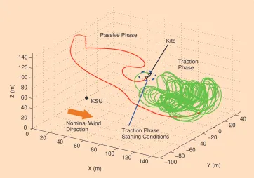
The traction phase begins when the kite is flying in a prescribed zone downwind of the KSU, at a suitable altitude ZI with a given line length r0 (see Figure 9).
When the traction phase starts, the kite flies as line length rincreases due to a positive value ˙rref of the line FIGURE 10 (a) Carousel configuration phases. The same rotor arm is depicted with three subse-quent angular values. The passive phase starts when the rotor arm reaches the angular position
0, and lasts until the rotation angle 3is reached. To maneuver the kite to a suitable position to begin the traction phase (highlighted in blue), the passive phase is divided into 3 subphases (gray, orange, and green) delimited by rotation angles 1and 2. (b) Kite trajectory with carousel config-uration. The kite follows figure-eight orbits, which maximize its speed during the traction phase (green), while during the passive phase (red) the airfoil speed is very low to reduce drag forces. The kite steering unit follows a circular trajectory at ground height, with radius R.
speed reference provided by the local motor controller. Since a traction force Fcis created on the kite lines, the
system generates mechanical power. The predictive control law computes the line angle ψ (see Figure 8) in order to vary Fc and thus optimize the aerodynamic
behavior of the kite for energy generation. The line angle ψ is obtained by varying laccording to (13) by imposing a setpoint on the desired line length achieved by the local motor controller.
The value of the reference line speed r˙ref is chosen as a
compromise between obtaining high traction force action
and high line winding speed. Basically, the stronger the wind, the higher the value of ˙rref that can be set while
obtaining high force values. The control system objective in the traction phase is to maximize the energy generated during the prediction interval [tk,tk+TP]. Since the
instantaneous generated mechanical power is
P(t)= ˙r(t)Fc(t), MPC minimizes the cost function
The traction phase ends when the length of the lines reach-es a given value rand the passive phase begins.
The passive phase is divided into three subphases. In the first subphase, the line speed ˙r(t) is controlled to smoothly decrease toward zero. The control objective is to move the kite into a zone with low values of θ and high values of |φ|(see Figure 7), where the effective wind speed
Weand force Fcare low and the kite can be recovered with
low energy expense. Then, in the second subphase, ˙r(t)is controlled to smoothly decrease from zero to a negative value, which provides a compromise between high rewinding speed and low force Fc. During this passive
subphase, the control objective is to minimize the energy spent to rewind the lines. This second subphase ends when the line length rreaches the desired minimum value. In the third passive subphase, r(t)˙ is controlled to smooth-ly increase toward zero from the previous negative set-point. The control objective is to move the kite in the traction phase starting zone. The passive phase ends when the starting conditions for the traction phase are reached.
Carousel Configuration Controller
In the carousel configuration (see figures 4 and 10), the torque Tc given by the carousel motor/generator is such
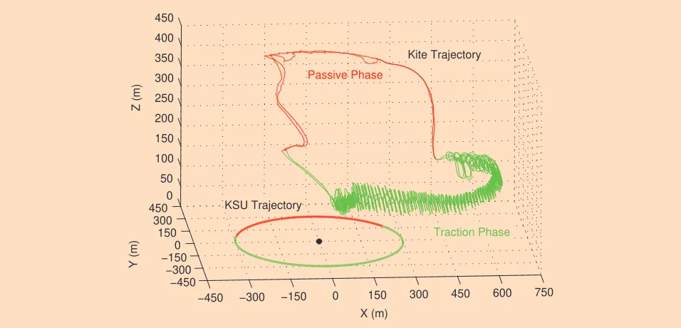
FIGURE 11 Simulation results for the yo-yo configuration. Kite trajec-tories are reported during the traction (green) and passive (red) phases of a complete yo-yo configuration cycle in the presence of wind turbulence. Note that the behavior is similar to Figure 9 despite the turbulence.
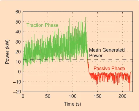
FIGURE 12 Simulated power obtained with the yo-yo configuration. A complete cycle is considered in the presence of wind turbulence. The instantaneous course of the generated power during the trac-tion phase (green) is reported together with the power spent for the kite recovery in the passive phase (red). The mean value of the power generated during the cycle, which is represented by a dashed line, is 11.8 kW. The corresponding generated energy is 2613 kJ per cycle.
0 50 100 150 200
FIGURE 13 Line speed reference imposed during a complete carousel cycle. The commanded line speed r˙(t)is chosen on the basis of simulation data to increase the mean generated power and to ensure that the lengths of the lines at the beginning of each cycle are the same.
Reference Line Winding Speed (m/s)
that the rotor moves at the constant reference angular speed ˙ref, which is chosen to optimize the net energy generated in the cycle. Since the angular speed is constant, each kite can be controlled independently, provided that the lines never collide. Thus, a single kite is considered in the following. The traction phase begins at the rotor angu-lar position =3, where the nominal wind direction is such that the kite can pull the rotor arm [see Figure 10(a)]. A suitable trajectory for the line speed ˙rduring the traction phase is set to further increase generated power. Recalling that mechanical power obtained at each instant is the sum of the effects given by line unrolling and rotor movement, MPC minimizes the cost function
J(tk)= − tk+Tp
tk ˙
r(τ )Fc(τ )+ ˙(τ )Tgen(τ )dτ . (21)
When the rotor arm reaches the angle 0, the kite can no longer pull the carousel, and the traction phase ends. Then, the passive phase starts, and the electric generator linked to the rotor acts as a motor to drag the carousel between angles 0 and 3. Meanwhile, the kite is moved to a suitable position for initiating the next traction phase. FIGURE 16 Power generated with the carousel configuration. Two com-plete cycles are considered in the presence of wind turbulence. The instantaneous course of the generated power during the traction phas-es (green) is reported together with the power required for the kite recovery in the passive phases (red). Note the nearly null values of energy usage during the passive phases. The mean value of the power generated during the two cycles is 621 kW and is represented by a dashed line. The corresponding generated energy is 234 MJ per cycle.
0 100 200 300 400 500 600 700
−500
0 500 1,000 1,500 2,000 2,500
Power (kW)
Mean Generated Power Traction Phase
Passive Phase Passive Phase Traction Phase
Carousel Angle Θ (°)
FIGURE 15 Figure-eight kite orbits during the traction phase for the carousel configuration. Such orbits are imposed by means of suit-able constraints on the angles θand φto avoid line wrapping.
150 200
250 300
−360 −340 −320 −300
−280 −260 −240
120 130 140 150 160 170 180 190
X (m)
Y (m)
Z (m)
FIGURE 14 Simulation results for the carousel configuration. Kite and kite steering unit trajectories are reported during traction (green) and passive (red) phases related to two complete cycles in the presence of turbulence. Note that, despite the turbulence, the trajectories show good repeatability.
−450 −300 −150 0 150 300 450 600 750
−450 −300 −150
0 150 300 450
0 50 100 150 200 250 300 350 400 450
X (m)
Y (m)
Z (m)
Passive Phase
KSU Trajectory
Kite Trajectory
The passive phase is divided into three subphases. Transitions between subphases are marked by suitable values 1 and 2 of the rotor angle [see Figure 10(a)], which are chosen to minimize the total energy spent
dur-ing the passive phase. In the first subphase, the control objective is to move each kite to a zone with a low value of θ [see figures 7 and 10(b)], where the effective wind speed We and pulling force component tangential to the
carousel Fcsinθsinφare much lower. At =1, the
sec-ond passive subphase begins, where the objective is to change the kite angular position φtoward φIto begin the traction phase. At =2, the third passive subphase begins, where the control objective is to increase the kite angle θ toward θII to prepare the generator for the sub-squent traction phase. For details, see [7].
SIMULATION RESULTS
Simulations of the KiteGen system were performed using the wind speed model
Wx(Z)=
0.04Z+8 m/s, if Z≤100 m, 0.0171(Z−100)+12 m/s, if Z>100 m.
(22)
The nominal wind speed is 8 m/s at 0 m altitude, while the wind speed grows linearly to 12 m/s at 100 m altitude and up to 17.2 m/s at 300 m altitude. Moreover, wind turbulence Wt is introduced, with uniformly distributed
random components along the inertial axes (X,Y,Z). The absolute value of each component of Wt ranges from 0
m/s to 3 m/s, which corresponds to 36% of the nominal wind speed at 100 m altitude.
Yo-Yo Configuration
For simulation, we consider a yo-yo configuration similar to the physical prototype. The numerical values of the kite TABLE 1 Model and control parameters of the simulated
yo-yo configuration. Note, in particular, the small characteristic area and low aerodynamic efficiency.
Symbol Numeric Value Description and Units
m 2.5 Kite mass (kg)
A 5 Characteristic area (m2)
ρ 1.2 Air density (kg/m3)
CL 1.2 Lift coefficient
CD 0.15 Drag coefficient
E= CL
CD 8 Aerodynamic efficiency
˙
r 1.5 Traction phase reference
for r˙(m/s) ˙
r −2.5 Passive phase reference for ˙
r(m/s)
Tc 0.1 Sample time (s)
Nc 1 Control horizon
Np 25 Prediction horizon
TABLE 2 State and input constraints and cycle starting and ending conditions for the simulated yo-yo configuration. The traction phase starts when θ≥θI, |φ− ¯φI| ≤5◦, and
r <rI. The passive phase starts when r >r¯. State and input constraints are imposed throughout the cycle.
Constraint Definition Constraint Description
θI =40◦ Traction phase starting conditions φI =0◦
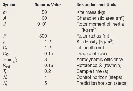
TABLE 3 Model and control parameters for the carousel configuration. Despite the low aerodynamic efficiency, this structure can generate a significant amount of energy as shown by the results reported in Figure 16.
Symbol Numeric Value Description and Units
m 50 Kite mass (kg)
A 100 Characteristic area (m2)
Jz 9108 Rotor moment of inertia (kg-m2)
R 300 Rotor radius (m)
ρ 1.2 Air density (kg/m3)
CL 1.2 Lift coefficient
CD 0.15 Drag coefficient
E= CL
CD 8 Aerodynamic efficiency
˙
ref 0.16 Reference ˙ (rev/min)
Tc 0.2 Sample time (s)
Nc 1 Control horizon (steps)
Np 5 Prediction horizon (steps)
TABLE 4 Objectives and starting conditions for the cycle phases and state and input constraints for the carousel configuration. In the passive phase, the controller is designed to drive θ to θI during the first subphase, φto φI during the second subphase, and θ to θI I during the third subphase. These values are chosen to minimize the energy used to return the kite to its position at the beginning of the traction phase. In particular, small values of θ and φ correspond to zones with low values of the effective wind speed and the tangential component of the pulling force Fc [see (14)]. State and input constraints are imposed throughout the cycle.
Constraint Definition Constraint Description
0=35◦ Passive phase starting condition
θI =20◦ First passive subphase objective
1=135◦ Second passive subphase starting condition
φI=140◦ Third passive subphase objective 2=150◦ Third passive subphase starting condition
θI I=50◦ Third passive subphase objective 3=165◦ Traction phase starting condition |θ (t)| ≤85◦ State constraint
model and control parameters are reported in Table 1, while Table 2 contains the state values for the start and end conditions of each phase as well as the values of the state and input constraints.
Figure 11 shows the trajectory of the kite, while the power generated during the cycle is reported in Fig-ure 12. The mean power is 11.8 kW, which corresponds to energy gener-ation of 2613 kJ per cycle.
Carousel Configuration
A carousel with a single KSU is considered. The model and con-trol parameters employed are reported in Table 3, while Table 4 contains the start and end condi-tions for each phase, as well as the values of the state and input con-straints. The line speed during the cycle is reported in Figure 13. This reference trajectory is chosen on the basis of the previous
simula-tion to maximize the mean generated power and to ensure that the length of the lines at the beginning of each cycle is the same.
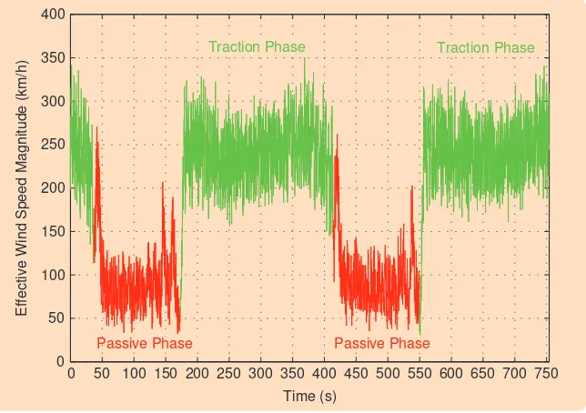
Figure 14 shows the trajectories of the kite and the control unit during two full cycles in the presence of ran-dom wind disturbances. Figure 15 depicts some orbits traced by the kite during the traction phase, while the power generated during the two cycles is reported in Figure 16. The mean power is 621 kW, and the generated energy is 234 MJ per cycle. Figure 17 depicts the course of the effective wind speed |We| (see the section “Kite
Generator Models” for details). It can be noted that dur-ing the traction phase the mean effective wind speed is about 14 times greater than the tangential speed of the rotor connected to the generator, which is 18 km/h. Since the fixed coordinate system (X,Y,Z) is defined on the basis of the nominal wind direction, a measurable change of the latter can be overcome by rotating the whole coordinate system (X,Y,Z), thus obtaining the same performance without changing either the control system parameters or the starting conditions of the vari-ous phases.
ACKNOWLEDGMENTS
KiteGen project is partially supported by Regione Piemonte under the Project “Controllo di aquiloni di potenza per la generazione eolica di energia” and by Min-istero dell’Università e della Ricerca of Italy under the National Project “Advanced control and identification techniques for innovative applications.”
REFERENCES
[1] “Renewables 2005: Global status report” Renewable Energy Policy Net-work, Worldwatch Institute, Wash. D.C., 2005 [Online]. Available: http://www.REN21.net
[2] M. Ippolito, “Smart control system exploiting the characteristics of gener-ic kites or airfoils to convert energy,” European patent 02840646, Dec. 2004. [3] M. Milanese and M. Ippolito “Automatic control system and process for the flight of kites,” International Patent PCT/IT2007/00325, May 2007. [4] M. Canale, L. Fagiano, M. Ippolito, and M. Milanese, “Control of tethered airfoils for a new class of wind energy generator,” in Proc. 45th IEEE Conf. Decision and Control, San Diego, CA, pp. 2006, 4020–4026.
[5] B. Houska and M. Diehl, “Optimal control for power gnerating kites,” in
Proc. 9th European Control Conf., Kos, Greece, 2007, pp. 3560–3567.
[6] A.R. Podgaets and W.J. Ockels, “Flight control of the high altitude wind power system,” in Proc. 7th Conf. Sustainable Applications Tropical Island States, Cape Canaveral, FL, 2007, pp. 125–130.
[7] M. Canale, L. Fagiano, M. Milanese, and M. Ippolito, “KiteGen project: Control as key technology for a quantum leap in wind energy generators,” in Proc. 26th American Control Conf., New York, 2007, pp. 3522–3528. [8] A. Betz, Introduction to the Theory of Flow Machines. New York: Pergamon, 1966. [9] M.L. Loyd, “Crosswind kite power,” J. Energy, vol. 4, no. 3, pp. 106–111, 1980.
[10] Danish Association of Wind Industry Web site [Online]. Available: www.windpower.org
[11] D.Q. Mayne, J.B. Rawlings, C.V. Rao, and P.O.M. Scokaert, “Con-strained model predictive control: Stability and optimality,” Automatica, vol. 36, pp. 789–814, 2000.
[12] M. Canale and M. Milanese, “FMPC: A fast implementation of model predictive control,” in Proc. 16th IFAC World Congress, Prague, Czech Repub-lic, July 2005.
[13] M. Canale, L. Fagiano, and M. Milanese, “Fast implementation of pre-dictive controllers using SM methodologies,” in Proc. 46th IEEE Conf. Deci-sion and Control, New Orleans, LA, 2007.
[14] M. Milanese and C. Novara, “Set membership identification of nonlinear systems,” Automatica, vol. 40, pp. 957–975, 2004.
[15] M. Milanese and C. Novara, “Structured set membership identification of nonlinear systems with application to vehicles with controlled suspensions,”
Control Eng. Practice, vol. 15, pp. 1–16, 2007.
[16] K. Hsu, M. Milanese, C. Novara, and K. Poolla, “Nonlinear virtual FIGURE 17 Simulated effective wind speed for the carousel configuration. The course of | We| during the traction subphases (green) and the passive subphases (red) is related to two com-plete carousel cycles. The average values are 250 km/h during the traction phase and 85 km/h during the passive phase.
0 50 100 150 200 250 300 350 400 450 500 550 600 650 700 750
Effective Wind Speed Magnitude (km/h)
Passive Phase Traction Phase
Passive Phase
sensors design from data,” in Proc. IFAC Symp. System Identification (SYSID), Newcastle, Australia, pp. 576–581, 2006.
[17] K. Hsu, M. Milanese, C. Novara, and K. Poolla, “Filter design from data: Direct vs. two-step approaches,” in Proc. 25th American Control Conf., Min-neapolis, MN, 2006, pp. 1606–1611.
[18] M. Diehl, “Real-time optimization for large scale nonlinear processes,” Ph.D. dissertation, University of Heidelberg, Germany, 2001 [Online]. Avail-able: http://www.iwr.uni-heidelberg.de/~Moritz.Diehl/DISSERTATION/ diehl_diss.pdf
AUTHOR INFORMATION
Massimo Canalereceived the Laurea degree in electronic engineering (1992) and the Ph.D. in systems engineering (1997), both from the Politecnico di Torino, Italy. From 1997 to 1998, he worked as a software engineer in the R&D department of Comau Robotics, Italy. Since 1998, he has been an assistant professor in the Dipartimento di Auto-matica e InforAuto-matica of the Politecnico di Torino. His research interests include robust control, model predictive control, set membership approximation, and application to automotive and aerospace problems.
Lorenzo Fagianoreceived the master’s degree in auto-motive engineering in 2004 from Politecnico di Torino, Italy. In 2005 he worked at Centro Ricerche Fiat, Italy, in the active vehicle systems area. Since January 2006 he has been a Ph.D. student at Politecnico di Torino. His main research interests include constrained robust and nonlinear control and set membership theory for control purposes, applied to vehicle stability control and the KiteGen project.