Cambridge University An Introduction To Statistical Signal Processing Jan 2005 ISBN 0521838606 pdf

(1)

An Introduction to

Statistical Signal Processing

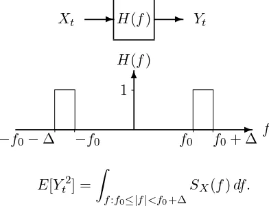
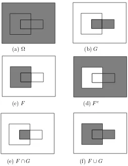
Pr(f ∈F) =P({ω :ω∈F}) =P(f−1(F)) f−1(F)

f

F

✲

November 22, 2003

(2)

(3)

An Introduction to

Statistical Signal Processing

Robert M. Gray and Lee D. Davisson

Information Systems Laboratory Department of Electrical Engineering

Stanford University and

Department of Electrical Engineering and Computer Science University of Maryland

(4)

c

(5)

(6)

(7)

The origins of this book lie in our earlier book Random Processes: A Mathematical Approach for Engineers, Prentice Hall, 1986. This book began as a second edition to the earlier book and the basic goal remains unchanged — to introduce the fundamental ideas and mechanics of random processes to engineers in a way that accurately reflects the underlying mathematics, but does not require an exten-sive mathematical background and does not belabor detailed general proofs when simple cases suffice to get the basic ideas across. In the years since the original book was published, however, it has evolved into something bearing little resemblence to its ancestor. Numerous improvements in the presentation of the material have been sug-gested by colleagues, students, teaching assistants, reviewers, and by our own teaching experience. The emphasis of the book shifted in-creasingly towards examples and a viewpoint that better reflected the title of the courses we taught for many years at Stanford University and at the University of Maryland using the book: An Introduction to Statistical Signal Processing. Much of the basic content of this course and of the fundamentals of random processes can be viewed as the analysis of statistical signal processing systems: typically one is given a probabilistic description for one random object, which can be considered as an input signal. An operation is applied to the in-put signal (signal processing) to produce a new random object, the

output signal. Fundamental issues include the nature of the basic probabilistic description and the derivation of the probabilistic

(13)

scription of the output signal given that of the input signal and a description of the particular operation performed. A perusal of the literature in statistical signal processing, communications, control, image and video processing, speech and audio processing, medical signal processing, geophysical signal processing, and classical statis-tical areas of time series analysis, classification and regression, and pattern recognition show a wide variety of probabilistic models for input processes and for operations on those processes, where the op-erations might be deterministic or random, natural or artificial, linear or nonlinear, digital or analog, or beneficial or harmful. An introduc-tory course focuses on the fundamentals underlying the analysis of such systems: the theories of probability, random processes, systems, and signal processing.

When the original book went out of print, the time seemed ripe to convert the manuscript from the prehistoric troff format to the widely used LA_{TEX format and to undertake a serious revision of the} book in the process. As the revision became more extensive, the title changed to match the course name and content. We reprint the original preface to provide some of the original motivation for the book, and then close this preface with a description of the goals sought during the many subsequent revisions.

Preface to Random Processes: An Introduction for Engineers

Nothing in nature is random . . . A thing appears random only through the incompleteness of our knowledge. — Spinoza,Ethics I

I do not believe that God rolls dice. — attributed to Einstein

(14)

too complex to compute in finite time. The computer itself may make errors due to power failures, lightning, or the general perfidy of inanimate objects. The experiment could take place in a remote location with the parameters unknown to the observer; for example, in a communication link, the transmitted message is unknowna pri-ori, for if it were not, there would be no need for communication. The results of the experiment could be reported by an unreliable witness — either incompetent or dishonest. For these and other reasons, it is useful to have a theory for the analysis and synthesis of processes that behave in a random or unpredictable manner. The goal is to construct mathematical models that lead to reasonably accurate pre-diction of the long-term average behavior of random processes. The theory should produce good estimates of the average behavior of real processes and thereby correct theoretical derivations with measur-able results.

(15)

Revisions

Through the years the original book has continually expanded to roughly double its original size to include more topics, examples, and problems. The material has been significantly reorganized in its grouping and presentation. Prerequisites and preliminaries have been moved to the appendices. Major additional material has been added on jointly Gaussian vectors, minimum mean squared error es-timation, detection and classification, filtering, and, most recently, mean square calculus and its applications to the analysis of contin-uous time processes. The index has been steadily expanded to ease navigation through the book. Numerous errors reported by reader email have been fixed and suggestions for clarifications and improve-ments incorporated.

This book is a work in progress. Revised versions will be made available through the World Wide Web page

http://ee.stanford.edu/~gray/sp.html .

The material is copyrighted by the University of Cambridge Press, but is freely available to any who wish to use it provided only that the contents of the entire text remain intact and to-gether. Comments, corrections, and suggestions should be sent to

rmgray@stanford.edu. Every effort will be made to fix typos and take suggestions into an account on at least an annual basis.

Acknowledgements

(16)

to the many readers ho have provided corrections and helpful sug-gestions through the Internet since the revisions began being posted. Particular thanks are due to Yariv Ephraim for his continuing thor-ough and helpful editorial commentary. Thanks also to Sridhar Ra-manujam, Raymond E. Rogers, Isabel Milho, Zohreh Azimifar, Dan Sebald, Muzaffer Kal, Greg Coxson, and several anonymous review-ers for Cambridge Univreview-ersity Press. Lastly, the first author would like to acknowledge his debt to his professors who taught him proba-bility theory and random processes, especially Al Drake and Wilbur B. Davenport, Jr. at MIT and Tom Pitcher at USC.

(17)

Glossary

{ } a collection of points satisfying some property, e.g., _{r:r _≤a_} is the collection of all real numbers less than or equal to a valuea

[ ] an interval of real points including the end points, e.g., for a_≤b [a, b] =_{r :a_≤r _≤b_}. Called aclosed interval.

( ) an interval of real points excluding the end points, e.g., for a_≤b (a, b) =_{r:a < r < b_}. Called an open interval. Note this is empty if a=b.

( ], [ ) denote intervals of real points including one endpoint and excluding the other, e.g., for a≤b (a, b] ={r:a < r≤b}, [a, b) ={r :a≤r < b}.

∅ the empty set, the set that contains no points.

∀ for all.

Ω the sample space or universal set, the set that contains all of the points.

#(F) the number of elements in a set F

(18)

exp the exponential function, exp(x) =∆ex_{, used for clarity when}_x

is complicated.

F Sigma-field or event space

B(Ω) Borel field of Ω, that is, the sigma-field of subsets of the real line generated by the intervals or the Cartesian product of a collection of such sigma-fields.

iff if and only if

l.i.m.limit in the mean

o(u) function of uthat goes to zero as u_→0 faster than u. P probability measure

PX distribution of a random variable or vectorX

pX probability mass function (pmf) of a random variable X

fX probability density function (pdf) of a random variable X

FX cumulative distribution function (cdf) of a random variable X

E(X) expectation of a random variable X

MX(ju) characteristic function of a random variable X

⊕addition modulo 2

1F(x) indicator function of a set F: 1F(x) = 1 if x∈F and 0

otherwise

Φ Phi function (Eq. (2.78))

(19)

Zk=∆{0,1,2, . . . , k−1}

Z+=∆{0,1,2, . . .}, the collection of nonnegative integers

(20)

(21)

1 Introduction

A random or stochastic process is a mathematical model for a phe-nomenon that evolves in time in an unpredictable manner from the viewpoint of the observer. The phenomenon may be a sequence of real-valued measurements of voltage or temperature, a binary data stream from a computer, a modulated binary data stream from a modem, a sequence of coin tosses, the daily Dow-Jones average, ra-diometer data or photographs from deep space probes, a sequence of images from a cable television, or any of an infinite number of possible sequences, waveforms, or signals of any imaginable type. It may be unpredictable due to such effects as interference or noise in a communication link or storage medium, or it may be an information-bearing signal-deterministic from the viewpoint of an observer at the transmitter but random to an observer at the receiver.

The theory of random processes quantifies the above notions so that one can construct mathematical models of real phenomena that are both tractable and meaningful in the sense of yielding useful predictions of future behavior. Tractability is required in order for the engineer (or anyone else) to be able to perform analyses and syntheses of random processes, perhaps with the aid of computers. The “meaningful” requirement is that the models must provide a reasonably good approximation of the actual phenomena. An over-simplified model may provide results and conclusions that do not apply to the real phenomenon being modeled. An overcomplicated one may constrain potential applications, render theory too difficult

(22)

to be useful, and strain available computational resources. Perhaps the most distinguishing characteristic between an average engineer and an outstanding engineer is the ability to derive effective models providing a good balance between complexity and accuracy.

Random processes usually occur in applications in the context of environments or systems whichchangethe processes to produce other processes. The intentional operation on a signal produced by one pro-cess, an “input signal,” to produce a new signal, an “output signal,” is generally referred to as signal processing, a topic easily illustrated by examples.

r _{A time varying voltage waveform is produced by a human speaking into}

a microphone or telephone. This signal can be modeled by a random pro-cess. This signal might be modulated for transmission, then it might be digitized and coded for transmission on a digital link. Noise in the digital link can cause errors in reconstructed bits, the bits can then be used to reconstruct the original signal within some fidelity. All of these operations on signals can be considered as signal processing, although the name is most commonly used for manmade operations such as modulation, digiti-zation, and coding, rather than the natural possibly unavoidable changes such as the addition of thermal noise or other changes out of our control.

r _{For very low bit rate digital speech communication applications, speech}

is sometimes converted into a model consisting of a simple linear filter (called an autoregressive filter) and an input process. The idea is that the parameters describing the model can be communicated with fewer bits than can the original signal, but the receiver can synthesize the human voice at the other end using the model so that it sounds very much like the original signal.

r _{Signals including image data transmitted from remote spacecraft are}

vir-tually buried in noise added to them on route and in the front end ampli-fiers of the receivers used to retrieve the signals. By suitably preparing the signals prior to transmission, by suitable filtering of the received sig-nal plus noise, and by suitable decision or estimation rules, high quality images are transmitted through this very poor channel.

r _{Signals produced by biomedical measuring devices can display specific}

behavior when a patient suddenly changes for the worse. Signal processing systems can look for these changes and warn medical personnel when suspicious behavior occurs.

(23)

can be automatically analyzed to locate possible anomolies indicating corrosion by looking for locally distinct random behavior.

How are these signals characterized? If the signals are random, how does one find stable behavior or structures to describe the pro-cesses? How do operations on these signals change them? How can one use observations based on random signals to make intelligent decisions regarding future behavior? All of these questions lead to aspects of the theory and application of random processes.

Courses and texts on random processes usually fall into either of two general and distinct categories. One category is the common engineering approach, which involves fairly elementary probability theory, standard undergraduate Riemann calculus, and a large dose of “cookbook” formulas — often with insufficient attention paid to conditions under which the formulas are valid. The results are of-ten justified by nonrigorous and occasionally mathematically inac-curate handwaving or intuitive plausibility arguments that may not reflect the actual underlying mathematical structure and may not be supportable by a precise proof. While intuitive arguments can be extremely valuable in providing insight into deep theoretical re-sults, they can be a handicap if they do not capture the essence of a rigorous proof.

A development of random processes that is insufficiently mathe-matical leaves the student ill prepared to generalize the techniques and results when faced with a real-world example not covered in the text. For example, if one is faced with the problem of designing signal processing equipment for predicting or communicating mea-surements being made for the first time by a space probe, how does one construct a mathematical model for the physical process that will be useful for analysis? If one encounters a process that is nei-ther stationary nor ergodic, what techniques still apply? Can the law of large numbers still be used to construct a useful model?

(24)

focuses on the structure common to all random processes. Even if an engineer is not directly involved in research, knowledge of the current literature can often provide useful ideas and techniques for tackling specific problems. Engineers unfamiliar with basic concepts such as

sigma-field and conditional expectation will find many potentially valuable references shrouded in mystery.

The other category of courses and texts on random processes is the typical mathematical approach, which requires an advanced mathe-matical background of real analysis, measure theory, and integration theory. This approach involves precise and careful theorem state-ments and proofs, and uses far more care to specify precisely the conditions required for a result to hold. Most engineers do not, how-ever, have the required mathematical background, and the extra care required in a completely rigorous development severely limits the number of topics that can be covered in a typical course — in par-ticular, the applications that are so important to engineers tend to be neglected. In addition, too much time is spent with the formal details, obscuring the often simple and elegant ideas behind a proof. Often little, if any, physical motivation for the topics is given.

This book attempts a compromise between the two approaches by giving the basic, elementary theory and a profusion of examples in the language and notation of the more advanced mathematical approaches. The intent is to make the crucial concepts clear in the traditional elementary cases, such as coin flipping, and thereby to emphasize the mathematical structure of all random processes in the simplest possible context. The structure is then further developed by numerous increasingly complex examples of random processes that have proved useful in systems analysis. The complicated examples are constructed from the simple examples by signal processing, that is, by using a simple process as an input to a system whose output is the more complicated process. This has the double advantage of describing the action of the system, the actual signal processing, and the interesting random process which is thereby produced. As one might suspect, signal processing also can be used to produce simple processes from complicated ones.

(25)

For example, the fundamental theorem of expectation is proved only for discrete random variables, where it is proved simply by a change of variables in a sum. The continuous analog is subsequently given without a careful proof, but with the explanation that it is simply the integral analog of the summation formula and hence can be viewed as a limiting form of the discrete result. As another example, only weak laws of large numbers are proved in detail in the mainstream of the text, but the strong law is treated in detail for a special case in a starred section. Starred sections are used to delve into other relatively advanced results, for example the use of mean square con-vergence ideas to make rigorous the notion of integration and filtering of continuous time processes.

By these means we strive to capture the spirit of important proofs without undue tedium and to make plausible the required assump-tions and constraints. This, in turn, should aid the student in deter-mining when certain tools do or do not apply and what additional tools might be necessary when new generalizations are required.

A distinct aspect of the mathematical viewpoint is the “grand ex-periment” view of random processes as being a probability measure on sequences (for discrete time) or waveforms (for continuous time) rather than being an infinity of smaller experiments representing in-dividual outcomes (called random variables) that are somehow glued together. From this point of view random variables are merely special cases of random processes. In fact, the grand experiment viewpoint was popular in the early days of applications of random processes to systems and was called the “ensemble” viewpoint in the work of Norbert Wiener and his students. By viewing the random process as a whole instead of as a collection of pieces, many basic ideas, such as stationarity and ergodicity, that characterize the dependence on time of probabilistic descriptions and the relation between time aver-ages and probabilistic averaver-ages are much easier to define and study. This also permits a more complete discussion of processes that vi-olate such probabilistic regularity requirements yet still have useful relations between time and probabilistic averages.

(26)

random processes, the basic results and their development and im-plications should be accessible, and the most common examples of random processes and classes of random processes should be familiar. In particular, the student should be well equipped to follow the gist of most arguments in the various Transactions of the IEEE dealing with random processes, including the IEEE Transactions on Signal Processing,IEEE Transactions on Image Processing,IEEE Transac-tions on Speech and Audio Processing,IEEE Transactions on Com-munications,IEEE Transactions on Control, andIEEE Transactions on Information Theory.

It also should be mentioned that the authors are electrical engi-neers and, as such, have written this text with an electrical engineer-ing flavor. However, the required knowledge of classical electrical engineering is slight, and engineers in other fields should be able to follow the material presented.

This book is intended to provide a one-quarter or one-semester course that develops the basic ideas and language of the theory of random processes and provides a rich collection of examples of com-monly encountered processes, properties, and calculations. Although in some cases these examples may seem somewhat artificial, they are chosen to illustrate the way engineers should think about random processes. They are selected for simplicity and conceptual content rather than to present the method of solution to some particular ap-plication. Sections that can be skimmed or omitted for the shorter one-quarter curriculum are marked with a star (⋆). Discrete time processes are given more emphasis than in many texts because they are simpler to handle and because they are of increasing practical im-portance in digital systems. For example, linear filter input/output relations are carefully developed for discrete time; then the contin-uous time analogs are obtained by replacing sums with integrals. The mathematical details underlying the continuous time results are found in a starred section.

(27)

simple processes. Extra tools are introduced as needed to develop properties of the examples.

The prerequisites for this book are elementary set theory, elemen-tary probability, and some familiarity with linear systems theory (Fourier analysis, convolution, discrete and continuous time linear filters, and transfer functions). The elementary set theory and prob-ability may be found, for example, in the classic text by Al Drake [18] or in the current MIT basic probability text by Bertsekas and Tsit-siklis [3]. The Fourier and linear systems material can by found in numerous texts, including Gray and Goodman [30]. Some of these basic topics are reviewed in this book in appendix A. These results are considered prerequisite as the pace and density of material would likely be overwhelming to someone not already familiar with the fun-damental ideas of probability such as probability mass and density functions (including the more common named distributions), com-puting probabilities, derived distributions, random variables, and ex-pectation. It has long been the authors’ experience that the students having the most difficulty with this material are those with little or no experience with elementary probability.

Organization of the Book

(28)

be viewed as forms of signal processing: each operates on “inputs,” which are the sample points of a probability space, and produces an “output,” which is the resulting sample value of the random variable, vector, or process. These output points together constitute an output sample space, which inherits its own probability measure from the structure of the measurement and the underlying experiment. As a result, many of the basic properties of random variables, vectors, and processes follow from those of probability spaces. Probability distributions are introduced along with probability mass functions, probability density functions, and cumulative distribution functions. The basic derived distribution method is described and demonstrated by example. A wide variety of examples of random variables, vectors, and processes are treated. Expectations are introduced briefly as a means of characterizing distributions and to provide some calculus practice.

Chapter 4 develops in depth the ideas of expectation — averages of random objects with respect to probability distributions. Also called probabilistic averages, statistical averages, and ensemble av-erages, expectations can be thought of as providing simple but im-portant parameters describing probability distributions. A variety of specific averages are considered, including mean, variance, char-acteristic functions, correlation, and covariance. Several examples of unconditional and conditional expectations and their properties and applications are provided. Perhaps the most important application is to the statement and proof of laws of large numbers or ergodic the-orems, which relate long term sample average behavior of random processes to expectations. In this chapter laws of large numbers are proved for simple, but important, classes of random processes. Other important applications of expectation arise in performing and ana-lyzing signal processing applications such as detecting, classifying, and estimating data. Minimum mean squared nonlinear and linear estimation of scalars and vectors is treated in some detail, showing the fundamental connections among conditional expectation, opti-mal estimation, and second order moments of random variables and vectors.

(29)

second-order moments — the mean and covariance — of a variety of random processes. The primary example is a form of derived distribution problem: if a given random process with known second-order moments is put into a linear system what are the second-second-order moments of the resulting output random process? This problem is treated for linear systems represented by convolutions and for linear modulation systems. Transform techniques are shown to provide a simplification in the computations, much like their ordinary role in elementary linear systems theory. Mean square convergence is revis-ited and several of its applications to the analysis of continuous time random processes are collected under the heading of mean square calculus. Included are a careful definition of integration and filtering of random processes, differentiation of random processes, and sam-pling and orghogonal expansions of random processes. In all of these examples the behavior of the second order moments determines the applicability of the results. The chapter closes with a development of several results from the theory of linear least-squares estimation. This provides an example of both the computation and the applica-tion of second-order moments.

(30)

Markov processes, Poisson and Gaussian processes, and the random telegraph wave process. We also briefly consider an example of a nonlinear system where the output random processes can at least be partially described — the exponential function of a Gaussian or Poisson process which models phase or frequency modulation. We close with examples of a type of “doubly stochastic” process — a compound process formed up by adding a random number of other random effects.

Appendix A sketches several prerequisite definitions and concepts from elementary set theory and linear systems theory using examples to be encountered later in the book. The first subject is crucial at an early stage and should be reviewed before proceeding to chapter 2. The second subject is not required until chapter 5, but it serves as a reminder of material with which the student should already be familiar. Elementary probability is not reviewed, as our basic devel-opment includes elementary probability. The review of prerequisite material in the appendix serves to collect together some notation and many definitions that will be used throughout the book. It is, however, only a brief review and cannot serve as a substitute for a complete course on the material. This chapter can be given as a first reading assignment and either skipped or skimmed briefly in class; lectures can proceed from an introduction, perhaps incorporating some preliminary material, directly to chapter 2.

Appendix B provides some scattered definitions and results needed in the book that detract from the main development, but may be of interest for background or detail. These fall primarily in the realm of calculus and range from the evaluation of common sums and integrals to a consideration of different definitions of integration. Many of the sums and integrals should be prerequisite material, but it has been the authors’ experience that many students have either forgotten or not seen many of the standard tricks. Hence several of the most im-portant techniques for probability and signal processing applications are included. Also in this appendix some background information on limits of double sums and the Lebesgue integral is provided.

(31)

func-tions and probability density funcfunc-tions along with their second order moments for reference.

The book concludes with an appendix suggesting supplementary reading, providing occasional historical notes, and delving deeper into some of the technical issues raised in the book. In that section we assemble references on additional background material as well as on books that pursue the various topics in more depth or on a more advanced level. We feel that these comments and references are supplementary to the development and that less clutter results by putting them in a single appendix rather than strewing them throughout the text. The section is intended as a guide for further study, not as an exhaustive description of the relevant literature, the latter goal being beyond the authors’ interests and stamina.

(32)

Probability

2.1 Introduction

The theory of random processes is a branch of probability theory and probability theory is a special case of the branch of mathematics known as measure theory. Probability theory and measure theory both concentrate on functions that assign real numbers to certain sets in an abstract space according to certain rules. These set functions can be viewed as measures of the size or weight of the sets. For example, the precise notion of area in two-dimensional Euclidean space and volume in three-dimensional space are both examples of measures on sets. Other measures on sets in three dimensions are mass and weight. Observe that from elementary calculus we can find volume by integrating a constant over the set. From physics we can find mass by integrating a mass density or summing point masses over a set. In both cases the set is a region of three-dimensional space. In a similar manner, probabilities will be computed by integrals of densities of probability or sums of “point masses” of probability.

Both probability theory and measure theory consider only nonneg-ative real-valued set functions. The value assigned by the function to a set is called the probability or themeasure of the set, respectively. The basic difference between probability theory and measure theory is that the former considers only set functions that are normalized in the sense of assigning the value of 1 to the entire abstract space, corresponding to the intuition that the abstract space contains every possible outcome of an experiment and hence should happen with

(33)

certainty or probability 1. Subsets of the space have some uncer-tainty and hence have probability less than 1.

Probability theory begins with the concept of a probability space, which is a collection of three items:

1. Anabstract spaceΩ, as encountered in appendix A, called asample space, which contains all distinguishable elementary outcomes or results of an experiment. These points might be names, numbers, or complicated signals.

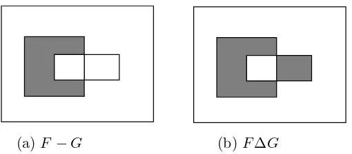
2. Anevent spaceorsigma-field _Fconsisting of a collection of subsets of the abstract space which we wish to consider as possible events and to which we wish to assign a probability. We require that the event space have an algebraic structure in the following sense: any finite or countably infinite sequence of set-theoretic operations (union, intersection, com-plementation, difference, symmetric difference) on events must produce other events.

3. Aprobability measure P — an assignment of a number between 0 and 1 to every event, that is, to every set in the event space. A probability measure must obey certain rules or axioms and will be computed by integrating or summing, analogously to area, volume, and mass compu-tations.

This chapter is devoted to developing the ideas underlying the triple (Ω,_F, P), which is collectively called a probability space or an experiment. Before making these ideas precise, however, several comments are in order.

(34)

ex-ample, if we spin a pointer and the outcome is known to be equally likely to be any number between 0 an 1, then the probability that any particular point such as .3781984637 or exactly 1/π occurs is 0 because there is an uncountable infinity of possible points, none more likely than the others. Hence knowing only that the probability of each and every point is zero, we would be hard pressed to make any meaningful inferences about the probabilities of other events such as the outcome being between 1/2 and 3/4. Writers of fiction (includ-ing Patrick O’Brian in his Aubrey-Maturin series) have often made much of the fact that extremely unlikely events often occur. One can say that zero probability events occur virtually all the time since the a priori probability that the universe will be exactly in a par-ticular configuration at 12:01AM Coordinated Universal Time (aka Greenwich Mean Time) is 0, yet the universe will indeed be in some configuration at that time.

The difficulty inherent in this example leads to a less natural as-pect of the probability space triumvirate — the fact that we must specify an event space or collection of subsets of our abstract space to which we wish to assign probabilities. In the example it is clear that taking the individual points and theircountable combinations is not enough (see also problem 2.3). On the other hand, why not just make the event space the class of all subsets of the abstract space? Why require the specification of which subsets are to be deemed suf-ficiently important to be blessed with the name “event”? In fact, this concern is one of the principal differences between elementary probability theory and advanced probability theory (and the point at which the student’s intuition frequently runs into trouble). When the abstract space is finite or even countably infinite, one can con-sider all possible subsets of the space to be events, and one can build a useful theory. When the abstract space is uncountably infinite,

(35)

however, as in the case of the space consisting of the real line or the unit interval, one cannot build a useful theory without constraining the subsets to which one will assign a probability. Roughly speak-ing, this is because probabilities of sets in uncountable spaces are found by integrating over sets, and some sets are simply too nasty to be integrated over. Although it is difficult to show, for such spaces there does not exist a reasonable and consistent means of assigning probabilities to all subsets without contradiction or without violat-ing desirable properties. In fact, it is so difficult to show that such “non-probability-measurable” subsets of the real line exist that we will not attempt to do so in this book. The reader should at least be aware of the problem so that the need for specifying an event space is understood. It also explains why the reader is likely to encounter phrases like “measurable sets” and “measurable functions” in the literature — some things are unmeasurable!

Thus a probability space must make explicit not just the elemen-tary outcomes or “finest-grain” outcomes that constitute our abstract space; it must also specify the collections of sets of these points to which we intend to assign probabilities. Subsets of the abstract space that do not belong to the event space will simply not have probabili-ties defined. The algebraic structure that we have postulated for the event space will ensure that if we take (countable) unions of events (corresponding to a logical “or”) or intersections of events (corre-sponding to a logical “and”), then the resulting sets are also events and hence will have probabilities. In fact, this is one of the main functions of probability theory: given a probabilistic description of a collection of events, find the probability of some new event formed by set-theoretic operations on the given events.

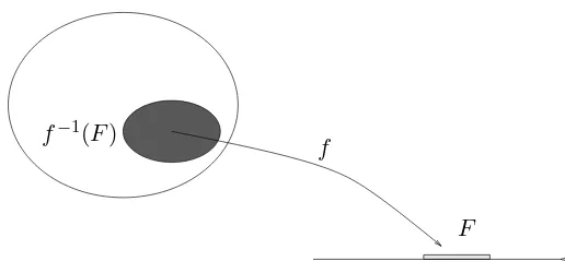
Up to this point the notion ofsignal processing has not been men-tioned. It enters at a fundamental level if one realizes that each in-dividual pointω _∈Ω produced in an experiment can be viewed as a

(36)

is the performing of some operation on the signal. In its simplest yet most general form this consists of applying some function or mapping or operation g to the signal or input ω to produce an output g(ω), which might be intended to guess some hidden parameter, extract useful information from noise, enhance an image, or any simple or complicated operation intended to produce a useful outcome. If we have a probabilistic description of the underlying experiment, then we should be able to derive a probabilistic description of the outcome of the signal processor. This, in fact, is the core problem of derived distributions, one of the fundamental tools of both probability the-ory and signal processing. In fact, this idea of defining functions on probability spaces is the foundation for the definition of random variables, random vectors, and random processes, which will inherit their basic properties from the underlying probability space, thereby yielding new probability spaces. Much of the theory of random pro-cesses and signal processing consists of developing the implications of certain operations on probability spaces: beginning with some probability space we form new ones by operations called variously mappings, filtering, sampling, coding, communicating, estimating, detecting, averaging, measuring, enhancing, predicting, smoothing, interpolating, classifying, analyzing or other names denoting linear or nonlinear operations. Stochastic systems theory is the combination of systems theory with probability theory. The essence of stochastic systems theory is the connection of a system to a probability space. Thus a precise formulation and a good understanding of probability spaces are prerequisites to a precise formulation and correct devel-opment of examples of random processes and stochastic systems.

Before proceeding to a careful development, several of the basic ideas are illustrated informally with simple examples.

2.2 Spinning Pointers and Flipping Coins

(37)

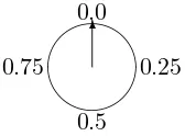
A Uniform Spinning Pointer

Suppose that Nature (or perhaps Tyche, the Greek Goddess of chance) spins a pointer in a circle as depicted in Figure 2.1. When

✫✪

✬✩0.0_✻

0.5

0.25 0.75

Figure 2.1. The Spinning Pointer

the pointer stops it can point to any number in the unit interval [0,1) =∆_{r : 0_≤r <1_}. We call [0,1) the sample space of our ex-periment and denote it by a capital Greek omega, Ω. What can we say about the probabilities or chances of particular events or out-comes occurring as a result of this experiment? The sorts of events of interest are things like “the pointer points to a number between 0 and .5” (which one would expect should have probability 0.5 if the wheel is indeed fair) or “the pointer does not lie between 0.75 and 1” (which should have a probability of 0.75). Two assumptions are implicit here. The first is that an “outcome” of the experiment or an “event” to which we can assign a probability is simply a subset of [0,1). The second assumption is that the probability of the pointer landing in any particular interval of the sample space is proportional to the length of the interval. This should seem reasonable if we in-deed believe the spinning pointer to be “fair” in the sense of not favoring any outcomes over any others. The bigger a region of the circle, the more likely the pointer is to end up in that region. We can formalize this by stating that for any interval [a, b] =_{r:a_≤r_≤b_} with 0_≤a_≤b <1 we have that the probability of the event “the pointer lands in the interval [a, b]” is

(38)

We do not have to restrict interest to intervals in order to define probabilities consistent with (2.1). The notion of the length of an interval can be made precise using calculus and simultaneously ex-tended to any subset of [0,1) by defining the probability P(F) of a set F _⊂[0,1) as

P(F)=∆

Z

F

f(r)dr, (2.2)

where f(r) = 1 for allr _∈[0,1). With this definition it is clear that for any 0_≤a < b_≤1 that

P([a, b]) =

Z b

a

f(r)dr=b₋a. (2.3) We could also arrive at effectively the same model by considering the sample space to be the entire real line, Ω =_ℜ= (∆ _−∞,_∞) and defining the pdf to be

f(r) =

(

1 if r_∈[0,1)

0 otherwise . (2.4)

The integral can also be expressed without specifying limits of inte-gration by using the indicator function of a set

1F(r)=∆ (

1 if r∈F

0 if r6∈F (2.5)

as

P(F)=∆

Z

1F(r)f(r)dr. (2.6)

(39)

interval, then both formulas must give the same numerical result — as they do in this example.

The second implicit assumption is that the integral exists in a well defined sense, that it can be evaluated using calculus. As surprising as it may seem to readers familiar only with typical engineering-oriented developments of Riemann integration, the integral of (2.2) is in fact not well defined for all subsets of [0,1). But we leave this detail for later and assume for the moment that we only encounter sets for which the integral (and hence the probability) is well defined. The function f(r) is called a probability density function or pdf

since it is a nonnegative point function that is integrated to compute total probability of a set, just as a mass density function is integrated over a region to compute the mass of a region in physics. Since in this examplef(r) is constant over a region, it is called auniform pdf.

The formula (2.2) for computing probability has many implica-tions, three of which merit comment at this point.

•Probabilities are nonnegative:

P(F)_≥0 for any F. (2.7)

This follows since integrating a nonnegative argument yields a non-negative result.

•The probability of the entire sample space is 1:

P(Ω) = 1. (2.8)

This follows since integrating 1 over the unit interval yields 1, but it has the intuitive interpretation that the probability that “something happens” is 1.

• The probability of the union of disjoint or mutually exclusive re-gions is the sum of the probabilities of the individual events:

(40)

This follows immediately from the properties of integration:

An alternative proof follows by observing that since F and G are disjoint, 1F∪G(r) = 1F(r) + 1G(r) and hence linearity of integration

This property is often called the additivity property of probability. The second proof makes it clear that additivity of probability is an immediate result of the linearity of integration, i.e., that the integral of the sum of two functions is the sum of the two integrals.

Repeated application of additivity for two events shows that for any finite collection _{Fk; k= 1,2, . . . , K} of disjoint events, i.e.,

showing that additivity is equivalent to finite additivity, the exten-sion of the additivity property from two to a finite collection of sets. Since additivity is a special case of finite additivity and it implies finite additivity, the two notions are equivalent and we can use them interchangably.

(41)

probability and will form three of the four axioms needed for a pre-cise development. It is tempting to call an assignmentP of numbers to subsets of a sample space aprobability measure if it satisfies these three properties, but we shall see that a fourth condition, which is crucial for having well behaved limits and asymptotics, will be needed to complete the definition. Pending this fourth condition, (2.2) defines a probability measure. In fact, this definition is com-plete in the simple case where the sample space Ω has only a finite number of points since in that case limits and asympotics become trivial. A sample space together with a probability measure provide a mathematical model for an experiment. This model is often called a probability space, but for the moment we shall stick to the less intimidating word ofexperiment.

Simple Properties

Several simple properties of probabilities can be derived from what we have so far. As particularly simple, but still important, examples, consider the following.

Assume that P is a set function defined on a sample space Ω that satisfies properties (2.7 – 2.9). Then

(a) P(Fc_{) = 1}₋_P₍_F₎ _.

(b) P(F)_≤1 .

(c) Let _∅be the null or empty set, then P(_∅) = 0 .

(d) If _{Fi; i= 1,2, . . . , K} is a finite partition of Ω, i.e., if Fi∩

Fk=∅ when i6=k and Si=1Fi= Ω, then

P(G) =

K X

i=1

P(G∩Fi) (2.11)

for any event G.

Proof (a) F∪Fc = Ω implies P(F∪Fc) = 1 (property (2.8)). F _∩Fc ₌_∅ _{implies 1 =}_P₍_F_∪_Fc_{) =}_P₍_F_{) +}_P₍_Fc_{) (property}

(2.9)).

(42)

(c) By property (2.8) and (a) above,P(Ωc) =P(∅) = 1−P(Ω) = 0.

(d) P(G) =P(G_∩Ω) =P(G_∩([

i

Fi)) =P( [

i

(G_∩Fi)) = X

i

P(G_∩Fi). ✷

Observe that although the null or empty set_∅ has probability 0, the converse is not true in that a set need not be empty just be-cause it has zero probability. In the uniform fair wheel example the set F =_{1/n:n= 1,2,3, . . ._} is not empty, but it does have probability zero. This follows roughly because for any finite N P({1/n:n= 2,3, . . . , N}) = 0 (since the integral of 1 over a finite set of points is zero) and therefore the limit as N → ∞ must also be zero, a “continuity of probability” idea that we shall later make rigorous.

A Single Coin Flip

The original example of a spinning wheel is continuous in that the sample space consists of a continuum of possible outcomes, all points in the unit interval. Sample spaces can also be discrete, as is the case of modeling a single flip of a “fair” coin with heads labeled “1” and tails labeled “0”, i.e., heads and tails are equally likely. The sample space in this example is Ω =_{0,1_} and the probability for any event or subset of Ω can be defined in a reasonable way by

P(F) =X

r∈F

p(r), (2.12)

or, equivalently,

P(F) =X1F(r)p(r), (2.13)

where now p(r) = 1/2 for each r _∈Ω. The function p is called a

(43)

when dealing with one-point or singleton sets, for example P({0}) =p(0)

P(_{1_}) =p(1).

This may seem too much work for such a little example, but keep in mind that the goal is a formulation that will work for far more complicated and interesting examples. This example is different from the spinning wheel in that the sample space is discrete instead of continuous and that the probabilities of events are defined by sums instead of integrals, as one should expect when doing discrete math. It is easy to verify, however, that the basic properties (2.7)–(2.9) hold in this case as well (since sums behave like integrals), which in turn implies that the simple properties(a)–(d) also hold.

A Single Coin Flip as Signal Processing

The coin flip example can also be derived in a very different way that provides our first example of signal processing. Consider again the spinning pointer so that the sample space is Ω and the probability measure P is described by (2.2) using a uniform pdf as in (2.4). Performing the experiment by spinning the pointer will yield some real numberr_∈[0,1). Define a measurementqmade on this outcome by

q(r) =

(

1 ifr∈[0,0.5]

0 ifr∈(0.5,1) . (2.14) This function can also be defined somewhat more economically in terms of an indicator function as

q(r) = 1_[0_,₀_._5](r). (2.15) This is an example of a quantizer, an operation that maps a con-tinuous value into a discrete value. Quantization is an example of

(44)

space. In this example Ωg ={0,1}. The dependence of a function

on its input space or domain of definition Ω and its output space or range Ωg,is often denoted byq : Ω→Ωg. Although introduced as

an example of simple signal processing, the usual name for a real-valued function defined on the sample space of a probability space is a random variable. We shall see in the next chapter that there is an extra technical condition on functions to merit this name, but that is a detail that can be postponed.

The output space Ωgcan be considered as a new sample space, the

space corresponding to the possible values seen by an observer of the output of the quantizer (an observer who might not have access to the original space). If we know both the probability measure on the input space and the function, then in theory we should be able to describe the probability measure that the output space inherits from the input space. Since the output space is discrete, it should be described by a pmf, saypq. Since there are only two points, we need only find the

value of pq(1) (or pq(0) since pq(0) +pq(1) = 1). An output of 1 is

seen if and only if the input sample point lies in [0,0.5], so it follows easily thatpq(1) =P([0,0.5]) =R₀0.5f(r), dr= 0.5, exactly the value

assumed for the fair coin flip model. The pmfpqimplies a probability

measure on the output space Ωg by

Pq(F) = X

ω∈F

pq(ω),

where the subscript q distinguishes the probability measure Pq on

the output space from the probability measureP on the input space. Note that we can define any other binary quantizer corresponding to an “unfair” or biased coin by changing the 0.5 to some other value.

(45)

space Ωq and probability measure Pq. Third, it is an example of a

common phenomenon that quite different models can result in identi-cal sample spaces and probability measures. Here the coin flip could be modeled in a directly given fashion by just describing the sam-ple space and the probability measure, or it can be modeled in an indirect fashion as a function (signal processing, random variable) on another experiment. This suggests, for example, that to study coin flips empirically we could either actually flip a fair coin, or we could spin a fair wheel and quantize the output. Although the sec-ond method seems more complicated, it is in fact extremely common since most random number generators (or pseudo-random number generators) strive to produce random numbers with a uniform dis-tribution on [0,1) and all other probability measures are produced by further signal processing. We have seen how to do this for a sim-ple coin flip. In fact any pdf or pmf can be generated in this way. (See problem 3.7.) The generation of uniform random numbers is both a science and an art. Most function roughly as follows. One begins with floating point number in (0,1) called the seed, say a, and uses another positive floating point number, say b, as a mul-tiplier. A sequence xn is then generated recursively as x0 =a and xn=b×xn−1 mod (1) for n= 1,2, . . ., that is, the fractional part of b×xn−1. If the two numbers a and b are suitably chosen then xn should appear to be uniform. (Try it!) In fact, since there are

only a finite number (albeit large) of possible numbers that can be represented on a digital computer, this algorithm must eventually repeat and hencexn must be a periodic sequence. As a result such a

(46)

Abstract vs. Concrete

It may seem strange that the axioms of probability deal with ap-parently abstract ideas of measures instead of corresponding phys-ical intuition. Physphys-ical intuition says that the probability tells you something about the fraction of times specific events will occur in a sequence of trials, such as the relative frequency of a pair of dice summing to seven in a sequence of many roles, or a decision algo-rithm correctly detecting a single binary symbol in the presence of noise in a transmitted data file. Such real world behavior can be quantified by the idea of a relative frequency, that is, suppose the output of the nth trial of a sequence of trials isxn and we wish to

know the relative frequency that xntakes on a particular value, say

a. Then given an infinite sequence of trials x=_{x0, x1, x2, . . .} we could define the relative frequency of ainx by

ra(x) = lim n→∞

number ofk_{∈ {}0,1, . . . , n₋1_}for which xk=a

n .

(47)

issue of the Annals of Probability, Volume 17, 1989. His contribu-tions to information theory, a shared interest area of the authors, are described in [11].) The axioms do, however, capture certain intuitive aspects of relative frequencies. Relative frequencies are nonnegative, the relative frequency of the entire set of possible outcomes is one, and relative frequencies are additive in the sense that the relative fre-quency of the symbolaor the symbolboccurring, ra∪b(x), is clearly

ra(x) +rb(x). Kolmogorov realized that beginning with simple

ax-ioms could lead to rigorous limiting results of the type needed, while there was no way to begin with the limiting results as part of the axioms. In fact it is the fourth axiom, a limiting version of additivity, that plays the key role in making the asymptotics work.

2.3 Probability Spaces

We now turn to a more thorough development of the ideas introduced in the previous section.

A sample space Ω is an abstract space, a nonempty collection of points or members or elements called sample points (or elementary events or elementary outcomes).

An event space (or sigma-field or sigma-algebra) _F of a sample space Ω is a nonempty collection of subsets of Ω called events with the following properties:

r

If F_{∈ F} ,then also Fc

∈ F , (2.17)

that is, if a given set is an event, then its complement must also be an event. Note that any particular subset of Ω may or may not be an event (review the quantizer example).

r

If for some finite n, Fi∈ F , i= 1,2, . . . , n, then also n

[

i=1

Fi∈ F , (2.18)

(48)

r

If Fi ∈ F , i= 1,2, . . . , then also ∞

[

i=1

Fi∈ F , (2.19)

that is, acountable union of events must also be an event.

We shall later see alternative ways of describing (2.19), but this form is the most common.

Eq. (2.18) can be considered as a special case of (2.19) since, for example, given a finite collection Fi; i= 1, . . . , N, we can construct

an infinite sequence of sets with the same union, e.g., given Fk,k=

1,2, . . . , N, construct an infinite sequence Gn with the same union

by choosing Gn=Fn for n= 1,2, . . . N and Gn=∅ otherwise. It

is convenient, however, to consider the finite case separately. If a collection of sets satisfies only (2.17) and (2.18) but not (2.19), then it is called a field or algebra of sets. For this reason, in elementary probability theory one often refers to “set algebra” or to the “algebra of events.” (Don’t worry about why (2.19) might not be satisfied.) Both (2.17) and (2.18) can be considered as “closure” properties; that is, an event space must be closed under complementation and unions in the sense that performing a sequence of complementations or unions of events must yield a set that is also in the collection, i.e., a set that is also an event. Observe also that (2.17), (2.18), and (A.11) imply that

Ω_{∈ F} , (2.20)

that is, the whole sample space considered as a set must be in _F; that is, it must be an event. Intuitively, Ω is the “certain event,” the event that “something happens.” Similarly, (2.20) and (2.17) imply that

∅ ∈ F, (2.21)

and hence the empty set must be in_F, corresponding to the intuitive event “nothing happens.”

(49)

F is in order. If the setF is a subset of Ω,then we write F _⊂Ω. If the subset F is also in the event space, then we write F ∈ F. Thus we use set inclusion when consideringF as a subset of an abstract space, and element inclusion when considering F as a member of the event space and hence as an event. Alternatively, the elements of Ω are points, and a collection of these points is a subset of Ω; but the elements of _F are sets — subsets of Ω, — and not points. A student should ponder the different natures of abstract spaces of points and event spaces consisting of sets until the reasons for set inclusion in the former and element inclusion in the latter space are clear. Consider especially the difference between an element of Ω and a subset of Ω that consists of a single point. The latter might

or might not be an element of F, the former is never an element of

F. Although the difference might seem to be merely semantics, the difference is important and should be thoroughly understood.

Ameasurable space (Ω,_F) is a pair consisting of a sample space Ω and an event space or sigma-field_Fof subsets of Ω.The strange name “measurable space” reflects the fact that we can assign a measure such as a probability measure, to such a space and thereby form a probability space or probability measure space.

Aprobability measureP on a measurable space (Ω,_F) is an assign-ment of a real number P(F) to every member F of the sigma-field (that is, to every event) such thatP obeys the following rules, which we refer to as theaxioms of probability.

Axiom 2.1

P(F)_≥0 for all F _{∈ F} (2.22)

i.e., no event has negative probability.

Axiom 2.2

P(Ω) = 1 (2.23)

(50)

Axiom 2.3 If Fi, i= 1,2, . . . , n are disjoint, then

Note that nothing has been said to the effect that probabilities must be sums or integrals, but the first three axioms should be rec-ognizable from the three basic properties of nonnegativity, normaliza-tion, and additivity encountered in the simple examples introduced in the introduction to this chapter where probabilities were defined by an integral of a pdf over a set or a sum of a pmf over a set. The axioms capture these properties in a general form and will be seen to include more general constructions, including multidimensional in-tegrals and combinations of inin-tegrals and sums. The fourth axiom can be viewed as an extra technical condition that must be included in order to get various limits to behave. Just as property (2.19) of an event space will later be seen to have an alternative statement in terms of limits of sets, the fourth axiom of probability, axiom 2.4, will be shown to have an alternative form in terms of explicit limits, a form providing an important continuity property of probability. Also as in the event space properties, the fourth axiom implies the third.

As with the defining properties of an event space, for the purposes of discussion we have listed separately the finite special case (2.24) of the general condition (2.25). The finite special case is all that is required for elementary discrete probability. The general condition is required to get a useful theory for continuous probability. A good way to think of these conditions is that they essentially describe probability measures as set functions defined by either summing or integrating over sets, or by some combination thereof. Hence much of probability theory is simply calculus, especially the evaluation of sums and integrals.

(51)

num-bers to elements of an event space of a sample space is a probability measureif and only if it satisfies all of the four axioms!

Aprobability space orexperiment is a triple (Ω,_F, P) consisting of a sample space Ω, an event space_Fof subsets of Ω, and a probability measureP defined for all members of_F.

Before developing each idea in more detail and providing several examples of each piece of a probability space, we pause to consider two simple examples of the complete construction. The first example is the simplest possible probability space and is commonly referred to as thetrivial probability space. Although useless for application, the model does serve a purpose, however, by showing that a well-defined model need not be interesting. The second example is essentially the simplest nontrivial probability space, a slight generalization of the fair coin flip permitting an unfair coin.

Examples

[2.0] Let Ω be any abstract space and let _F =_{Ω,_∅}; that is, _F consists of exactly two sets — the sample space (everything) and the empty set (nothing). This is called the trivial event space. This is a model of an experiment where only two events are possi-ble: “Something happens” or “nothing happens” — not a very in-teresting description. There is only one possible probability mea-sure for this measurable space: P(Ω) = 1 and P(_∅) = 0.(Why?) This probability measure meets the required rules that define a probability measure; they can be directly verified since there are only two possible events. Equations (2.22) and (2.23) are obvi-ous. Equations (2.24) and (2.25) follow since the only possible values forFi are Ω and∅. At most one of theFi can be Ω. If one

of the Fi is Ω, then both sides of the equality are 1. Otherwise,

both sides are 0.

[2.1] Let Ω ={0,1}. Let F ={{0},{1},Ω ={0,1},∅}. Since F

(52)

this example. What is it?) Define the set function P by

P(F) =

      

1₋pif F =_{0_} p if F =_{1_} 0 if F =_∅ 1 if F = Ω,

wherep_∈[0,1] is a fixed parameter. (Ifp= 0 orp= 1 the space becomes trivial.) It is easily verified that P satisfies the axioms of probability and hence is a probability measure. Therefore (Ω,_F, P) is a probability space. Note that we had to give the value ofP(F) forall eventsF, a construction that would clearly be absurd for large sample spaces. Note also that the choice of P(F) is not unique for the given measurable space (Ω,_F); we could have chosen any value in [0,1] for P(_{1_}) and used the axioms to complete the definition.

The preceding example is the simplest nontrivial example of a probability space and provides a rigorous mathematical model for applications such as the binary transmission of a single bit or for the flipping of a single biased coin once. It therefore provides a complete and rigorous mathematical model for the single coin flip of the introduction.

We now develop in more detail properties and examples of the three components of probability spaces: sample spaces, event spaces, and probability measures.

2.3.1 Sample Spaces

Intuitively, a sample space is a listing of all conceivable finest-grain, distinguishable outcomes of an experiment to be modeled by a prob-ability space. Mathematically it is just an abstract space.

Examples

[2.2] A finite space Ω ={ak;k= 1,2, . . . , K}. Specific examples

are the binary space_{0,1_} and the finite space of integers _Zk=∆

{0,1,2, . . . , k₋1_}.

(53)

sequence{ak}. Specific examples are the space of all nonnegative

integers_{0,1,2, . . ._},which we denote by_Z+, and the space of all integers _{. . . ,₋2,₋1,0,1,2, . . ._}, which we denote by _Z. Other examples are the space of all rational numbers, the space of all even integers, and the space of all periodic sequences of integers. Both examples [2.2] and [2.3] are called discrete spaces. Spaces with finite or countably infinite numbers of elements are called dis-crete spaces.

[2.4] An interval of the real line ℜ, for example, Ω = (a, b). We might consider an open interval (a, b), a closed interval [a, b], a half-open interval [a, b) or (a, b], or even the entire real line ℜ

itself. (See appendix A for details on these different types of intervals.)

Spaces such as example [2.4] that are not discrete are said to be

continuous. In some cases it is more accurate to think of spaces as being a mixture of discrete and continuous parts, e.g., the space Ω = (1,2)_{∪ {}4_} consisting of a continuous interval and an isolated point. Such spaces can usually be handled by treating the discrete and continuous components separately.

[2.5] A space consisting ofk₋dimensional vectors with coordinates taking values in one of the previously described spaces. A useful notation for such vector spaces is a product space. Let A de-note one of the abstract spaces previously considered. Define the Cartesian productAk _by

Ak={all vectors a= (a0, a1, . . . , ak−1) withai ∈A} .

Thus, for example, ℜk _is _k₋_{dimensional Euclidean space.} _{₀_,₁_}k

is the space of all binary k₋tuples, that is, the space of all k−dimensional binary vectors. As particular examples, {0,1}2 ₌

(54)

Alternative notations for a Cartesian product space are

Y

i∈Zk Ai =

k_Y−1

i=0 Ai ,

where again the Ai are all replicas or copies of A, that is, where

Ai =A,alli.Other notations for such a finite-dimensional Cartesian

product are

×i∈ZkAi =×

k−1

i=0Ai =Ak .

This and other product spaces will prove to be a useful means of describing abstract spaces which model sequences of elements from another abstract space.

Observe that a finite-dimensional vector space constructed from a discrete space is also discrete since if one can count the number of possible values one coordinate can assume, then one can count the number of possible values that a finite number of coordinates can assume.

[2.6] A space consisting of infinite sequences drawn from one of the examples [2.2] through [2.4]. Points in this space are often called discrete time signals. This is also a product space. Let A be a sample space and letAi be replicas or copies of A. We will

consider both one-sided and two-sided infinite products to model sequences with and without a finite origin, respectively. Define the two-sided space

Y

i∈Z

Ai={all sequences {ai;i=. . . ,−1,0,1, . . .};ai∈Ai} ,

and the one-sided space

Y

i∈Z+

Ai ={all sequences {ai;i= 0,1, . . .};ai ∈Ai} .

These two spaces are also denoted byQ∞_i₌_−∞Ai or ×∞i=−∞Ai and Q_∞

i=0Ai or ×∞i=0Ai, respectively.

The two spaces under discussion are often calledsequence spaces.