Enterprise Data Workflows with Cascading by Paco Nathan
Copyright © 2013 Paco Nathan. All rights reserved.
Printed in the United States of America.
Published by O’Reilly Media, Inc., 1005 Gravenstein Highway North, Sebastopol, CA 95472.
O’Reilly books may be purchased for educational, business, or sales promotional use. Online editions are also available for most titles (http://my.safaribooksonline.com). For more information, contact our corporate/ institutional sales department: 800-998-9938 or [email protected].
Editors: Mike Loukides and Courtney Nash Production Editor: Kristen Borg
Copyeditor: Kim Cofer Proofreader: Julie Van Keuren
Indexer: Paco Nathan Cover Designer: Randy Comer Interior Designer: David Futato Illustrator: Rebecca Demarest
July 2013: First Edition
Revision History for the First Edition: 2013-07-10: First release
See http://oreilly.com/catalog/errata.csp?isbn=9781449358723 for release details.
Nutshell Handbook, the Nutshell Handbook logo, and the O’Reilly logo are registered trademarks of O’Reilly Media, Inc. Enterprise Data Workflows with Cascading, the image of an Atlantic cod, and related trade dress are trademarks of O’Reilly Media, Inc.
Many of the designations used by manufacturers and sellers to distinguish their products are claimed as trademarks. Where those designations appear in this book, and O’Reilly Media, Inc., was aware of a trade‐ mark claim, the designations have been printed in caps or initial caps.
While every precaution has been taken in the preparation of this book, the publisher and author assume no responsibility for errors or omissions, or for damages resulting from the use of the information contained herein.
ISBN: 978-1-449-35872-3
Table of Contents
Preface. . . vii
1. Getting Started. . . 1
Programming Environment Setup 1
Example 1: Simplest Possible App in Cascading 3
Build and Run 4
Cascading Taxonomy 6
Example 2: The Ubiquitous Word Count 8
Flow Diagrams 10
Predictability at Scale 14
2. Extending Pipe Assemblies. . . 17
Example 3: Customized Operations 17
Scrubbing Tokens 21
Example 4: Replicated Joins 22
Stop Words and Replicated Joins 25
Comparing with Apache Pig 27
Comparing with Apache Hive 29
3. Test-Driven Development. . . 33
Example 5: TF-IDF Implementation 33
Example 6: TF-IDF with Testing 41
A Word or Two About Testing 48
4. Scalding—A Scala DSL for Cascading. . . 51
Why Use Scalding? 51
Getting Started with Scalding 52
Example 3 in Scalding: Word Count with Customized Operations 54
A Word or Two about Functional Programming 57
Key Points of the Recommender Workflow 137
A. Troubleshooting Workflows. . . 141
Index. . . 145
Preface
Requirements
Throughout this book, we will explore Cascading and related open source projects in the context of brief programming examples. Familiarity with Java programming is re‐ quired. We’ll show additional code in Clojure, Scala, SQL, and R. The sample apps are all available in source code repositories on GitHub. These sample apps are intended to run on a laptop (Linux, Unix, and Mac OS X, but not Windows) using Apache Hadoop in standalone mode. Each example is built so that it will run efficiently with a large data set on a large cluster, but setting new world records on Hadoop isn’t our agenda. Our intent here is to introduce a new way of thinking about how Enterprise apps get designed. We will show how to get started with Cascading and discuss best practices for Enterprise data workflows.
Enterprise Data Workflows
Cascading provides an open source API for writing Enterprise-scale apps on top of Apache Hadoop and other Big Data frameworks. In production use now for five years (as of 2013Q1), Cascading apps run at hundreds of different companies and in several verticals, which include finance, retail, health care, and transportation. Case studies have been published about large deployments at Williams-Sonoma, Twitter, Etsy, Airbnb, Square, The Climate Corporation, Nokia, Factual, uSwitch, Trulia, Yieldbot, and the Harvard School of Public Health. Typical use cases for Cascading include large
extract/transform/load (ETL) jobs, reporting, web crawlers, anti-fraud classifiers, social recommender systems, retail pricing, climate analysis, geolocation, genomics, plus a variety of other kinds of machine learning and optimization problems.
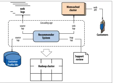
Keep in mind that Apache Hadoop rarely if ever gets used in isolation. Generally speak‐ ing, apps that run on Hadoop must consume data from a variety of sources, and in turn they produce data that must be used in other frameworks. For example, a hypothetical social recommender shown in Figure P-1 combines input data from customer profiles
in a distributed database plus log files from a cluster of web servers, then moves its recommendations out to Memcached to be served through an API. Cascading encom‐ passes the schema and dependencies for each of those components in a workflow—data sources for input, business logic in the application, the flows that define parallelism, rules for handling exceptions, data sinks for end uses, etc. The problem at hand is much more complex than simply a sequence of Hadoop job steps.
Figure P-1. Example social recommender
Moreover, while Cascading has been closely associated with Hadoop, it is not tightly coupled to it. Flow planners exist for other topologies beyond Hadoop, such as in-memory data grids for real-time workloads. That way a given app could compute some parts of a workflow in batch and some in real time, while representing a consistent “unit of work” for scheduling, accounting, monitoring, etc. The system integration of many different frameworks means that Cascading apps define comprehensive workflows.
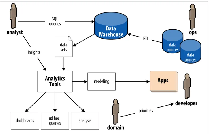
An analyst typically would make a SQL query in a data warehouse such as Oracle or Teradata to pull a data set. That data set might be used directly for a pivot tables in Excel for ad hoc queries, or as a data cube going into a business intelligence (BI) server such as Microstrategy for reporting. In turn, a stakeholder such as a product owner would consume that analysis via dashboards, spreadsheets, or presentations. Alternatively, an analyst might use the data in an analytics platform such as SAS for predictive modeling, which gets handed off to a developer for building an application. Ops runs the apps, manages the data warehouse (among other things), and oversees ETL jobs that load data from other sources. Note that in this diagram there are multiple components—data warehouse, BI server, analytics platform, ETL—which have relatively expensive licens‐ ing and require relatively expensive hardware. Generally these apps “scale up” by pur‐ chasing larger and more expensive licenses and hardware.
Figure P-2. Enterprise data workflows, pre-Hadoop
Circa late 1997 there was an inflection point, after which a handful of pioneering Internet companies such as Amazon and eBay began using “machine data”—that is to say, data gleaned from distributed logs that had mostly been ignored before—to build large-scale data apps based on clusters of “commodity” hardware. Prices for disk-based storage and commodity servers dropped considerably, while many uses for large clusters began to arise. Apache Hadoop derives from the MapReduce project at Google, which was part of this inflection point. More than a decade later, we see widespread adoption of Hadoop in Enterprise use cases. On one hand, generally these use cases “scale out” by running
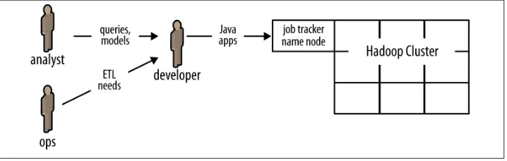
workloads in parallel on clusters of commodity hardware, leveraging mostly open source software. That mitigates the rising cost of licenses and proprietary hardware as data rates grow enormously. On the other hand, this practice imposes an interesting change in business process: notice how in Figure P-3 the developers with Hadoop ex‐ pertise become a new kind of bottleneck for analysts and operations.
Enterprise adoption of Apache Hadoop, driven by huge savings and opportunities for new kinds of large-scale data apps, has increased the need for experienced Hadoop programmers disproportionately. There’s been a big push to train current engineers and analysts and to recruit skilled talent. However, the skills required to write large Hadoop apps directly in Java are difficult to learn for most developers and far outside the norm of expectations for analysts. Consequently the approach of attempting to retrain current staff does not scale very well. Meanwhile, companies are finding that the process of hiring expert Hadoop programmers is somewhere in the range of difficult to impossible. That creates a dilemma for staffing, as Enterprise rushes to embrace Big Data and Apache Hadoop: SQL analysts are available and relatively less expensive than Hadoop experts.
Figure P-3. Enterprise data workflows, with Hadoop
An alternative approach is to use an abstraction layer on top of Hadoop—one that fits well with existing Java practices. Several leading IT publications have described Cas‐ cading in those terms, for example:
Management can really go out and build a team around folks that are already very ex‐ perienced with Java. Switching over to this is really a very short exercise.
— Thor Olavsrud
Cascading recently added support for ANSI SQL through a library called Lingual. An‐ other library called Pattern supports the Predictive Model Markup Language (PMML), which is used by most major analytics and BI platforms to export data mining models. Through these extensions, Cascading provides greater access to Hadoop re‐ sources for the more traditional analysts as well as Java developers. Meanwhile, other projects atop Cascading—such as Scalding (based on Scala) and Cascalog (based on Clojure)—are extending highly sophisticated software engineering practices to Big Da‐ ta. For example, Cascalog provides features for test-driven development (TDD) of En‐ terprise data workflows.
Complexity, More So Than Bigness
It’s important to note that a tension exists between complexity and innovation, which is ultimately driven by scale. Closely related to that dynamic, a spectrum emerges about technologies that manage data, ranging from “conservatism” to “liberalism.”
Consider that technology start-ups rarely follow a straight path from initial concept to success. Instead they tend to pivot through different approaches and priorities before finding market traction. The book Lean Startup by Eric Ries (Crown Business) articu‐ lates the process in detail. Flexibility is key to avoiding disaster; one of the biggest lia‐ bilities a start-up faces is that it cannot change rapidly enough to pivot toward potential success—or that it will run out of money before doing so. Many start-ups choose to use Ruby on Rails, Node.js, Python, or PHP because of the flexibility those scripting lan‐ guages allow.
On one hand, technology start-ups tend to crave complexity; they want and need the problems associated with having many millions of customers. Providing services so mainstream and vital that regulatory concerns come into play is typically a nice problem to have. Most start-ups will never reach that stage of business or that level of complexity in their apps; however, many will try to innovate their way toward it. A start-up typically wants no impediments—that is where the “liberalism” aspects come in. In many ways, Facebook exemplifies this approach; the company emerged through intense customer experimentation, and it retains that aspect of a start-up even after enormous growth.
A Political Spectrum for Programming
Consider the arguments this article presents about software “liberalism” versus “con‐ servatism”:
Just as in real-world politics, software conservatism and liberalism are radically different world views. Make no mistake: they are at odds. They have opposing value systems, priorities, core beliefs and motivations. These value systems clash at design time, at implementation time, at diagnostic time, at recovery time. They get along like green eggs and ham.
— Steve Yegge
Notes from the Mystery Machine Bus (2012)
This spectrum is encountered in the use of Big Data frameworks, too. On the “liberalism” end of the spectrum, there are mostly start-ups—plus a few notable large firms, such as Facebook. On the “conservatism” end of the spectrum there is mostly Enterprise—plus a few notable start-ups, such as The Climate Corporation.
On the other hand, you probably don’t want your bank to run customer experiments on your checking account, not anytime soon. Enterprise differs from start-ups because of the complexities of large, existing business units. Keeping a business running smooth‐ ly is a complex problem, especially in the context of aggressive competition and rapidly changing markets. Generally there are large liabilities for mishandling data: regulatory and compliance issues, bad publicity, loss of revenue streams, potential litigation, stock market reactions, etc. Enterprise firms typically want no surprises, and predictability is key to avoiding disaster. That is where the “conservatism” aspects come in.
Enterprise organizations must live with complexity 24/7, but they crave innovation. Your bank, your airline, your hospital, the power plant on the other side of town—those have risk profiles based on “conservatism.” Computing environments in Enterprise IT typically use Java virtual machine (JVM) languages such as Java, Scala, Clojure, etc. In some cases scripting languages are banned entirely. Recognize that this argument is not about political views; rather, it’s about how to approach complexity. The risk profile for a business vertical tends to have a lot of influence on its best practices.
duction, scripting tools such as Hive and Pig have been popular Hadoop abstractions. They provide lots of flexibility and work well for performing ad hoc queries at scale.
Relatively speaking, circa 2013, it is not difficult to load a few terabytes of unstructured data into an Apache Hadoop cluster and then run SQL-like queries in Hive. Difficulties emerge when you must make frequent updates to the data, or schedule mission-critical apps, or run many apps simultaneously. Also, as workflows integrate Hive apps with other frameworks outside of Hadoop, those apps gain additional complexity: parts of the business logic are declared in SQL, while other parts are represented in another programming language and paradigm. Developing and debugging complex workflows becomes expensive for Enterprise organizations, because each issue may require hours or even days before its context can be reproduced within a test environment.
A fundamental issue is that the difficulty of operating at scale is not so much a matter of bigness in data; rather, it’s a matter of managing complexity within the data. For com‐ panies that are just starting to embrace Big Data, the software development lifecycle (SDLC) itself becomes the hard problem to solve. That difficulty is compounded by the fact that hiring and training programmers to write MapReduce code directly is already a bitter pill for most companies.
Table P-1 shows a pattern of migration, from the typical “legacy” toolsets used for large-scale batch workflows—such as J2EE and SQL—into the adoption of Apache Hadoop and related frameworks for Big Data.
Table P-1. Migration of batch toolsets
Workflow Legacy Manage complexity Early adopter Pipelines J2EE Cascading Pig
Queries SQL Lingual (ANSI SQL) Hive Predictive models SAS Pattern (PMML) Mahout
As more Enterprise organizations move to use Apache Hadoop for their apps, typical Hadoop workloads shift from early adopter needs toward mission-critical operations. Typical risk profiles are shifting toward “conservatism” in programming environments. Cascading provides a popular solution for defining and managing Enterprise data workflows. It provides predictability and accountability for the physical plan of a work‐ flow and mitigates difficulties in handling exceptions, troubleshooting bugs, optimizing code, testing at scale, etc.
Also keep in mind the issue of how the needs for a start-up business evolve over time. For the firms working on the “liberalism” end of this spectrum, as they grow there is often a need to migrate into toolsets that are more toward the “conservatism” end. A large code base that has been originally written based on using Pig or Hive can be considerably difficult to migrate. Alternatively, writing that same functionality in a
framework such as Cascalog would provide flexibility for the early phase of the start-up, while mitigating complexity as the business grows.
Origins of the Cascading API
In the mid-2000s, Chris Wensel was a system architect at an Enterprise firm known for its data products, working on a custom search engine for case law. He had been working with open source code from the Nutch project, which gave him early hands-on expe‐ rience with popular spin-offs from Nutch: Lucene and Hadoop. On one hand, Wensel recognized that Hadoop had great potential for indexing large sets of documents, which was core business at his company. On the other hand, Wensel could foresee that coding in Hadoop’s MapReduce API directly would be difficult for many programmers to learn and would not likely scale for widespread adoption.
Moreover, the requirements for Enterprise firms to adopt Hadoop—or for any pro‐ gramming abstraction atop Hadoop—would be on the “conservatism” end of the spec‐ trum. For example, indexing case law involves large, complex ETL workflows, with substantial liability if incorrect data gets propagated through the workflow and down‐ stream to users. Those apps must be solid, data provenance must be auditable, workflow responses to failure modes must be deterministic, etc. In this case, Ops would not allow solutions based on scripting languages.
Late in 2007, Wensel began to write Cascading as an open source application framework for Java developers to develop robust apps on Hadoop, quickly and easily. From the beginning, the project was intended to provide a set of abstractions in terms of database primitives and the analogy of “plumbing.” Cascading addresses complexity while em‐ bodying the “conservatism” of Enterprise IT best practices. The abstraction is effective on several levels: capturing business logic, implementing complex algorithms, specify‐ ing system dependencies, projecting capacity needs, etc. In addition to the Java API, support for several other languages has been built atop Cascading, as shown in
Figure P-4.
Formally speaking, Cascading represents a pattern language for the business process management of Enterprise data workflows. Pattern languages provide structured meth‐ ods for solving large, complex design problems—where the syntax of the language pro‐ motes use of best practices. For example, the “plumbing” metaphor of pipes and oper‐ ators in Cascading helps indicate which algorithms should be used at particular points, which architectural trade-offs are appropriate, where frameworks need to be integrated, etc.
errors long before an app begins to consume expensive resources on a large cluster. Or in another sense, long before an app begins to propagate the wrong results downstream.
Figure P-4. Cascading technology stack
Also in late 2007, Yahoo! Research moved the Pig project to the Apache Incubator. Pig and Cascading are interesting to contrast, because newcomers to Hadoop technologies often compare the two. Pig represents a data manipulation language (DML), which provides a query algebra atop Hadoop. It is not an API for a JVM language, nor does it specify a pattern language. Another important distinction is that Pig attempts to per‐ form optimizations on a logical plan, whereas Cascading uses a physical plan only. The former is great for early adopter use cases, ad hoc queries, and less complex applications. The latter is great for Enterprise data workflows, where IT places a big premium on “no surprises.”
In the five years since 2007, there have been two major releases of Cascading and hun‐ dreds of Enterprise deployments. Programming with the Cascading API can be done in a variety of JVM-based languages: Java, Scala, Clojure, Python (Jython), and Ruby (JRuby). Of these, Scala and Clojure have become the most popular for large deployments.
Several other open source projects, such as DSLs, taps, libraries, etc., have been written based on Cascading sponsored by Twitter, Etsy, eBay, Climate, Square, etc.—such as Scalding and Cascalog—which help integrate with a variety of different frameworks.
Scalding @Twitter
It’s no wonder that Scala and Clojure have become the most popular languages used for commercial Cascading deployments. These languages are relatively flexible and dy‐ namic for developers to use. Both include REPLs for interactive development, and both leverage functional programming. Yet they produce apps that tend toward the “con‐ servatism” end of the spectrum, according to Yegge’s argument.
Scalding provides a pipe abstraction that is easy to understand. Scalding and Scala in general have excellent features for developing large-scale data services. Cascalog apps are built from logical predicates—functions that represent queries, which in turn act much like unit tests. Software engineering practices for TDD, fault-tolerant workflows, etc., become simple to use at very large scale.
As a case in point, the revenue quality team at Twitter is quite different from Eric Ries’s
Lean Startup notion. The “lean” approach of pivoting toward initial customer adoption is great for start-ups, and potentially for larger organizations as well. However, initial customer adoption is not exactly an existential crisis for a large, popular social network. Instead they work with data at immense scale and complexity, with a mission to monetize social interactions among a very large, highly active community. Outages of the mission-critical apps that power Twitter’s advertising servers would pose substantial risks to the business.
This team has standardized on Scalding for their apps. They’ve also written extensions, such as the Matrix API for very large-scale work in linear algebra and machine learning, so that complex apps can be expressed in a minimal amount of Scala code. All the while, those apps leverage the tooling that comes along with JVM use in large clusters, and conforms to Enterprise-scale requirements from Ops.
Using Code Examples
Most of the code samples in this book draw from the GitHub repository for Cascading:
• https://github.com/Cascading
We also show code based on these third-party GitHub repositories:
• https://github.com/nathanmarz/cascalog
Safari® Books Online
Safari Books Online is an on-demand digital library that delivers expert content in both book and video form from the world’s lead‐ ing authors in technology and business.
Technology professionals, software developers, web designers, and business and crea‐ tive professionals use Safari Books Online as their primary resource for research, prob‐ lem solving, learning, and certification training.
Safari Books Online offers a range of product mixes and pricing programs for organi‐ zations, government agencies, and individuals. Subscribers have access to thousands of books, training videos, and prepublication manuscripts in one fully searchable database from publishers like O’Reilly Media, Prentice Hall Professional, Addison-Wesley Pro‐ fessional, Microsoft Press, Sams, Que, Peachpit Press, Focal Press, Cisco Press, John Wiley & Sons, Syngress, Morgan Kaufmann, IBM Redbooks, Packt, Adobe Press, FT Press, Apress, Manning, New Riders, McGraw-Hill, Jones & Bartlett, Course Technol‐ ogy, and dozens more. For more information about Safari Books Online, please visit us
online.
How to Contact Us
Please address comments and questions concerning this book to the publisher:
O’Reilly Media, Inc.
1005 Gravenstein Highway North Sebastopol, CA 95472
800-998-9938 (in the United States or Canada) 707-829-0515 (international or local)
707-829-0104 (fax)
We have a web page for this book, where we list errata, examples, and any additional information. You can access this page at http://oreil.ly/enterprise-data-workflows. To comment or ask technical questions about this book, send email to bookques [email protected].
For more information about our books, courses, conferences, and news, see our website at http://www.oreilly.com.
Find us on Facebook: http://facebook.com/oreilly
Follow us on Twitter: http://twitter.com/oreillymedia
Watch us on YouTube: http://www.youtube.com/oreillymedia
Kudos
CHAPTER 1
Getting Started
Programming Environment Setup
The following code examples show how to write apps in Cascading. The apps are in‐ tended to run on a laptop using Apache Hadoop in standalone mode, on a laptop run‐ ning Linux or Unix (including Mac OS X). If you are using a Windows-based laptop, then many of these examples will not work, and generally speaking Hadoop does not behave well under Cygwin. However, you could run Linux, etc., in a virtual machine. Also, these examples are not intended to show how to set up and run a Hadoop cluster. There are other good resources about that—see Hadoop: The Definitive Guide by Tom White (O’Reilly).
First, you will need to have a few platforms and tools installed:
Java
• Version 1.6.x was used to create these examples.
• Get the JDK, not the JRE.
• Install according to vendor instructions.
Apache Hadoop
• Version 1.0.x is needed for Cascading 2.x used in these examples.
• Be sure to install for “Standalone Operation.”
Gradle
• Version 1.3 or later is required for some examples in this book.
• Install according to vendor instructions.
Git
• There are other ways to get code, but these examples show use of Git.
• Install according to vendor instructions.
Our use of Gradle and Git implies that these commands will be downloading JARs, checking code repos, etc., so you will need an Internet connection for most of the ex‐ amples in this book.
Next, set up your command-line environment. You will need to have the following environment variables set properly, according to the installation instructions for each project and depending on your operating system:
• JAVA_HOME
• HADOOP_HOME
• GRADLE_HOME
Assuming that the installers for both Java and Git have placed binaries in the appropriate directories, now extend your PATH definition for the other tools that depend on Java:
$ export PATH=$PATH:$HADOOP_HOME/bin:$GRADLE_HOME/bin
OK, now for some tests. Try the following command lines to verify that your installations worked:
$ java -version $ hadoop -version $ gradle --version $ git --version
Each command should print its version information. If there are problems, most likely you’ll get errors at this stage. Don’t worry if you see a warning like the following—that is a known behavior in Apache Hadoop:
Warning: $HADOOP_HOME is deprecated.
It’s a great idea to create an account on GitHub, too. An account is not required to run the sample apps in this book. However, it will help you follow project updates for the example code, participate within the developer community, ask questions, etc.
Also note that you do not need to install Cascading. Certainly you can, but the Gradle build scripts used in these examples will pull the appropriate version of Cascading from the Conjars Maven repo automatically. Conjars has lots of interesting JARs for related projects—take a peek sometime.
$ git clone git://github.com/Cascading/Impatient.git
Once that completes, connect into the part1 subdirectory. You’re ready to begin pro‐ gramming in Cascading.
Example 1: Simplest Possible App in Cascading
The first item on our agenda is how to write a simple Cascading app. The goal is clear and concise: create the simplest possible app in Cascading while following best practices. This app will copy a file, potentially a very large file, in parallel—in other words, it performs a distributed copy. No bangs, no whistles, just good solid code.
First, we create a source tap to specify the input data. That data happens to be formatted as tab-separated values (TSV) with a header row, which the TextDelimited data scheme handles.
String inPath = args[ 0 ];
Tap inTap = new Hfs( new TextDelimited( true, "\t" ), inPath );
Next we create a sink tap to specify the output data, which will also be in TSV format:
String outPath = args[ 1 ];
Tap outTap = new Hfs( new TextDelimited( true, "\t" ), outPath );
Then we create a pipe to connect the taps:
PipecopyPipe = new Pipe( "copy" );
Here comes the fun part. Get your tool belt ready, because we need to do a little plumb‐ ing. Connect the taps and the pipe to create a flow:
FlowDef flowDef = FlowDef.flowDef() .addSource( copyPipe, inTap ) .addTailSink( copyPipe, outTap );
The notion of a workflow lives at the heart of Cascading. Instead of thinking in terms of map and reduce phases in a Hadoop job step, Cascading developers define workflows and business processes as if they were doing plumbing work.
Enterprise data workflows tend to use lots of job steps. Those job steps are connected and have dependencies, specified as a directed acyclic graph (DAG). Cascading uses
FlowDef objects to define how a flow—that is to say, a portion of the DAG—must be connected. A pipe must connect to both a source and a sink. Done and done. That defines the simplest flow possible.
Now that we have a flow defined, one last line of code invokes the planner on it. Planning a flow is akin to the physical plan for a query in SQL. The planner verifies that the correct fields are available for each operation, that the sequence of operations makes sense, and that all of the pipes and taps are connected in some meaningful way. If the planner
detects any problems, it will throw exceptions long before the app gets submitted to the Hadoop cluster.
flowConnector.connect( flowDef ).complete();
Generally, these Cascading source lines go into a static main method in a Main class. Look in the part1/src/main/java/impatient/ directory, in the Main.java file, where this is already done. You should be good to go.
Each different kind of computing framework is called a topology, and each must have its own planner class. This example code uses the HadoopFlowConnector class to invoke the flow planner, which generates the Hadoop job steps needed to implement the flow. Cascading performs that work on the client side, and then submits those jobs to the Hadoop cluster and tracks their status.
If you want to read in more detail about the classes in the Cascading API that were used, see the Cascading User Guide and JavaDoc.
Build and Run
Cascading uses Gradle to build the JAR for an app. The build script for “Example 1: Simplest Possible App in Cascading” is in build.gradle:
apply plugin: 'java'
mavenRepo name: 'conjars', url: 'http://conjars.org/repo/'
}
ext.cascadingVersion = '2.1.0'
dependencies {
compile( group: 'cascading', name: 'cascading-core', version: cascadingVersion ) compile( group: 'cascading', name: 'cascading-hadoop', version: cascadingVersion ) }
jar {
description = "Assembles a Hadoop ready jar file"
doFirst {
into( 'lib' ) {
from configurations.compile }
manifest {
attributes( "Main-Class": "impatient/Main" ) }
}
Notice the reference to a Maven repo called http://conjars.org/repo/ in the build script. That is how Gradle accesses the appropriate version of Cascading, pulling from the open source project’s Conjars public Maven repo.
Books about Gradle and Maven
For more information about using Gradle and Maven, check out these books:
• Building and Testing with Gradle: Understanding Next-Generation Builds by Tim Berglund and Matthew McCullough (O’Reilly)
• Maven: The Definitive Guide by Sonatype Company (O’Reilly)
To build this sample app from a command line, run Gradle:
$ gradle clean jar
Note that each Cascading app gets compiled into a single JAR file. That is to say, it includes all of the app’s business logic, system integrations, unit tests, assertions, ex‐ ception handling, etc. The principle is “Same JAR, any scale.” After building a Cascading app as a JAR, a developer typically runs it on a laptop for unit tests and other validation using relatively small-scale data. Once those tests are confirmed, the JAR typically moves into continuous integration (CI) on a staging cluster using moderate-scale data. After passing CI, Enterprise IT environments generally place a tested JAR into a Maven repository as a new version of the app that Ops will schedule for production use with the full data sets.
What you should have at this point is a JAR file that is ready to run. Before running it, be sure to clear the output directory. Apache Hadoop insists on this when you’re running in standalone mode. To be clear, these examples are working with input and output paths that are in the local filesystem, not HDFS.
Now run the app:
$ rm -rf output
$ hadoop jar ./build/libs/impatient.jar data/rain.txt output/rain
Notice how those command-line arguments (actual parameters) align with the args[]
array (formal parameters) in the source. In the first argument, the source tap loads from the input file data/rain.txt, which contains text from search results about “rain shadow.” Each line is supposed to represent a different document. The first two lines look like this:
doc_id text
doc01 A rain shadow is a dry area on the lee back side of a mountainous area.
Input tuples get copied, TSV row by TSV row, to the sink tap. The second argument specifies that the sink tap be written to the output/rain output, which is organized as a partition file. You can verify that those lines got copied by viewing the text output, for example:
$ head -2 output/rain/part-00000 doc_id text
doc01 A rain shadow is a dry area on the lee back side of a mountainous area.
For quick reference, the source code, input data, and a log for this example are listed in a GitHub gist. If the log of your run looks terribly different, something is probably not set up correctly. There are multiple ways to interact with the Cascading developer com‐ munity. You can post a note on the cascading-user email forum. Plenty of experienced Cascading users are discussing taps and pipes and flows there, and they are eager to help. Or you can visit one of the Cascading user group meetings.
Cascading Taxonomy
Conceptually, a “flow diagram” for this first example is shown in Figure 1-1. Our simplest app possible copies lines of text from file “A” to file “B.” The “M” and “R” labels represent the map and reduce phases, respectively. As the flow diagram shows, it uses one job step in Apache Hadoop: only one map and no reduce needed. The implementation is a brief Java program, 10 lines long.
Wait—10 lines of code to copy a file? That seems excessive; certainly this same work could be performed in much quicker ways, such as using the cp command on Linux. However, keep in mind that Cascading is about the “plumbing” required to make En‐ terprise apps robust. There is some overhead in the setup, but those lines of code won’t change much as an app’s complexity grows. That overhead helps provide for the prin‐ ciple of “Same JAR, any scale.”
Let’s take a look at the components of a Cascading app. Figure 1-2 shows a taxonomy that starts with apps at the top level. An app has a unique signature and is versioned, and it includes one or more flows. Optionally, those flows may be organized into
cascades, which are collections of flows without dependencies on one another, so that they may be run in parallel.
a large data set can become enormous. Again, that addresses a more “conservatism” aspect of Cascading.
Figure 1-1. Flow diagram for “Example 1: Simplest Possible App in Cascading”
Figure 1-2. Cascading taxonomy
We’ve already introduced the use of pipes. Each assembly of pipes has a head and a tail. We bind taps to pipes to create a flow; so source taps get bound to the heads of pipes for input data, and sink taps to the tails of pipes for output data. That is the functional graph. Any unconnected pipes and taps will cause the planner to throw exceptions.
The physical plan of a flow results in a dependency graph of one or more steps. Formally speaking, that is a directed acyclic graph (DAG). At runtime, data flows through the DAG as streams of key/value tuples.
The steps created by a Hadoop flow planner, for example, correspond to the job steps that run on the Hadoop cluster. Within each step there may be multiple phases, e.g., the map phase or reduce phase in Hadoop. Also, each step is composed of slices. These are the most granular “unit of work” in a Cascading app, such that collections of slices can be parallelized. In Hadoop these slices correspond to the tasks executing in task slots.
That’s it in a nutshell, how the proverbial neck bone gets connected to the collarbone in Cascading.
Example 2: The Ubiquitous Word Count
The first example showed how to do a file copy in Cascading. Let’s take that code and stretch it a bit further. Undoubtedly you’ve seen Word Count before. We’d feel remiss if we did not provide an example.
Word Count serves as a “Hello World” for Hadoop apps. In other words, this simple program provides a great test case for parallel processing:
• It requires a minimal amount of code.
• It demonstrates use of both symbolic and numeric values.
• It shows a dependency graph of tuples as an abstraction.
• It is not many steps away from useful search indexing.
When a distributed computing framework can run Word Count in parallel at scale, it can handle much larger and more interesting algorithms. Along the way, we’ll show how to use a few more Cascading operations, plus show how to generate a flow diagram as a visualization.
Starting from the source code directory that you cloned in Git, connect into the part2
subdirectory. For quick reference, the source code and a log for this example are listed
in a GitHub gist. Input data remains the same as in the earlier code.
Note that the names of the taps have changed. Instead of inTap and outTap, we’re using
docTap and wcTap now. We’ll be adding more taps, so this will help us have more de‐ scriptive names. This makes it simpler to follow all the plumbing.
Fields token = new Fields( "token" );
Out of that pipe, we get a tuple stream of token values. One benefit of using a regex is that it’s simple to change. We can handle more complex cases of splitting tokens without having to rewrite the generator.
Next, we use a GroupBy to count the occurrences of each token:
PipewcPipe = new Pipe( "wc", docPipe );
wcPipe = new GroupBy( wcPipe, token );
wcPipe = new Every( wcPipe, Fields.ALL, new Count(), Fields.ALL );
Notice that we’ve used Each and Every to perform operations within the pipe assembly. The difference between these two is that an Each operates on individual tuples so that it takes Function operations. An Every operates on groups of tuples so that it takes
Aggregator or Buffer operations—in this case the GroupBy performed an aggregation. The different ways of inserting operations serve to categorize the different built-in op‐ erations in Cascading. They also illustrate how the pattern language syntax guides the development of workflows.
From that wcPipe we get a resulting tuple stream of token and count for the output. Again, we connect the plumbing with a FlowDef:
FlowDef flowDef = FlowDef.flowDef() .setName( "wc" )
.addSource( docPipe, docTap ) .addTailSink( wcPipe, wcTap );
Finally, we generate a DOT file to depict the Cascading flow graphically. You can load the DOT file into OmniGraffle or Visio. Those diagrams are really helpful for trouble‐ shooting workflows in Cascading:
Flow wcFlow = flowConnector.connect( flowDef );
wcFlow.writeDOT( "dot/wc.dot" );
wcFlow.complete();
This code is already in the part2/src/main/java/impatient/ directory, in the Main.java
file. To build it:
$ gradle clean jar
Then to run it:
$ rm -rf output
$ hadoop jar ./build/libs/impatient.jar data/rain.txt output/wc
This second example uses the same input from the first example, but we expect different output. The sink tap writes to the partition file output/wc, and the first 10 lines (including a header) should look like this:
$ head output/wc/part-00000 token count 9 A 3 Australia 1 Broken 1 California's 1 DVD 1 Death 1 Land 1 Secrets 1
Again, a GitHub gist shows building and running the sample app. If your run looks terribly different, something is probably not set up correctly. Ask the Cascading devel‐ oper community how to troubleshoot for your environment.
So that’s our Word Count example. Eighteen lines of yummy goodness.
Flow Diagrams
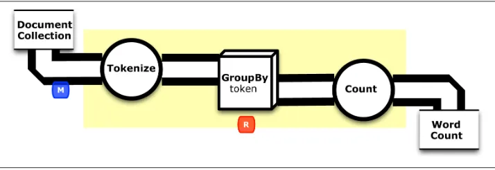
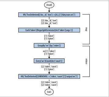
Conceptually, we can examine a workflow as a stylized flow diagram. This helps visualize the “plumbing” metaphor by using a design that removes low-level details. Figure 1-3
shows one of these for “Example 2: The Ubiquitous Word Count”. Formally speaking, this diagram represents a DAG.
Figure 1-3. Conceptual flow diagram for “Example 2: The Ubiquitous Word Count”
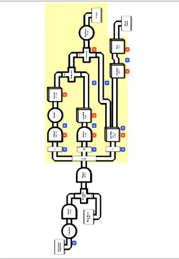
Meanwhile the Cascading code in “Example 2: The Ubiquitous Word Count” writes a
you ask other Cascading developers for help debugging an issue, don’t be surprised when their first request is to see your app’s flow diagram.
Figure 1-4. Annotated flow diagram for “Example 2: The Ubiquitous Word Count”
From a high-level perspective, “Example 2: The Ubiquitous Word Count” differs from
“Example 1: Simplest Possible App in Cascading” in two ways:
• Source and sink taps are more specific.
• Three operators have been added to the pipe assembly.
Although several lines of Java source code changed, in pattern language terms we can express the difference between the apps simply as those two points. That’s a powerful benefit of using the “plumbing” metaphor.
First let’s consider how the source and sink taps were redefined to be more specific. Instead of simply describing a generic “Source” or “File A,” now we’ve defined the source
tap as a collection of text documents. Instead of “Sink” or “File B,” now we’ve defined the sink tap to produce word count tuples—the desired end result. Those changes in the taps began to reference fields in the tuple stream. The source tap in both examples was based on TextDelimited with parameters so that it reads a TSV file and uses the header line to assign field names. “Example 1: Simplest Possible App in Cascading”
ignored the fields by simply copying data tuple by tuple. “Example 2: The Ubiquitous Word Count” begins to reference fields by name, which introduces the notion of scheme
—imposing some expectation of structure on otherwise unstructured data.
The change in taps also added semantics to the workflow, specifying requirements for added operations needed to reach the desired results. Let’s consider the new Cascading operations that were added to the pipe assembly in “Example 1: Simplest Possible App in Cascading”: Tokenize, GroupBy, and Count. The first one, Tokenize, transforms the input data tuples, splitting lines of text into a stream of tokens. That transform represents the “T” in ETL. The second operation, GroupBy, performs an aggregation. In terms of Hadoop, this causes a reduce with token as a key. The third operation, Count, gets applied to each aggregation—counting the values for each token key, i.e., the number of in‐ stances of each token in the stream.
The deltas between “Example 1: Simplest Possible App in Cascading” and “Example 2: The Ubiquitous Word Count” illustrate important aspects of Cascading. Consider how data tuples flow through a pipe assembly, getting routed through familiar data operators such as GroupBy, Count, etc. Each flow must be connected to a source of data as its input and a sink as its output. The sink tap for one flow may in turn become a source tap for another flow. Each flow defines a DAG that Cascading uses to infer schema from un‐ structured data.
• Ensure that necessary fields are available to operations that require them—based on tuple scheme.
• Apply transformations to help optimize the app—e.g., moving code from reduce into map.
• Track data provenance across different sources and sinks—understand the pro‐ ducer/consumer relationship of data products.
• Annotate the DAG with metrics from each step, across the history of an app’s in‐ stances—capacity planning, notifications for data drops, etc.
• Identify or predict bottlenecks, e.g., key/value skew as the shape of the input data changes—troubleshoot apps.
Those capabilities address important concerns in Enterprise IT and stand as key points by which Cascading differentiates itself from other Hadoop abstraction layers.
Another subtle point concerns the use of taps. On one hand, data taps are available for integrating Cascading with several other popular data frameworks, including Memcached, HBase, Cassandra, etc. Several popular data serialization systems are sup‐ ported, such as Apache Thrift, Avro, Kyro, etc. Looking at the conceptual flow diagram, our workflow could be using any of a variety of different data frameworks and seriali‐ zation systems. That could apply equally well to SQL query result sets via JDBC or to data coming from Cassandra via Thrift. It wouldn’t be difficult to modify the code in
“Example 2: The Ubiquitous Word Count” to set those details based on configuration parameters. To wit, the taps generalize many physical aspects of the data so that we can leverage patterns.
On the other hand, taps also help manage complexity at scale. Our code in “Example 2: The Ubiquitous Word Count” could be run on a laptop in Hadoop’s “standalone” mode to process a small file such as rain.txt, which is a mere 510 bytes. The same code could be run on a 1,000-node Hadoop cluster to process several petabytes of the Internet Archives’ Wayback Machine.
Taps are agnostic about scale, because the underlying topology (Hadoop) uses paral‐ lelism to handle very large data. Generally speaking, Cascading apps handle scale-out into larger and larger data sets by changing the parameters used to define taps. Taps themselves are formal parameters that specify placeholders for input and output data. When a Cascading app runs, its actual parameters specify the actual data to be used— whether those are HDFS partition files, HBase data objects, Memcached key/values, etc. We call these tap identifiers. They are effectively uniform resource identifiers (URIs) for connecting through protocols such as HDFS, JDBC, etc. A dependency graph of tap identifiers and the history of app instances that produced or consumed them is analo‐ gous to a catalog in relational databases.
Predictability at Scale
The code in “Example 1: Simplest Possible App in Cascading” showed how to move data from point A to point B. That was simply a distributed file copy—loading data via distributed tasks, or the “L” in ETL.
A copy example may seem trivial, and it may seem like Cascading is overkill for that. However, moving important data from point A to point B reliably can be a crucial job to perform. This helps illustrate one of the key reasons to use Cascading.
Consider an analogy of building a small Ferris wheel. With a little bit of imagination and some background in welding, a person could cobble one together using old bicycle parts. In fact, those DIY Ferris wheels show up at events such as Maker Faire. Starting out, a person might construct a little Ferris wheel, just for demo. It might not hold anything larger than hamsters, but it’s not a hard problem. With a bit more skill, a person could probably build a somewhat larger instance, one that’s big enough for small chil‐ dren to ride.
Ask yourself this: how robust would a DIY Ferris wheel need to be before you let your kids ride on it? That’s precisely part of the challenge at an event like Maker Faire. Makers must be able to build a device such as a Ferris wheel out of spare bicycle parts that is robust enough that strangers will let their kids ride. Let’s hope those welds were made using best practices and good materials, to avoid catastrophes.
That’s a key reason why Cascading was created. When you need to move a few gigabytes from point A to point B, it’s probably simple enough to write a Bash script, or just use a single command-line copy. When your work requires some reshaping of the data, then a few lines of Python will probably work fine. Run that Python code from your Bash script and you’re done.
That’s a great approach, when it fits the use case requirements. However, suppose you’re not moving just gigabytes. Suppose you’re moving terabytes, or petabytes. Bash scripts won’t get you very far. Also think about this: suppose an app not only needs to move data from point A to point B, but it must follow the required best practices of an En‐ terprise IT shop. Millions of dollars and potentially even some jobs ride on the fact that the app performs correctly. Day in and day out. That’s not unlike trusting a Ferris wheel made by strangers; the users want to make sure it wasn’t just built out of spare bicycle parts by some amateur welder. Robustness is key.
With Cascading, you can package your entire MapReduce application, including its orchestration and testing, within a single JAR file. You define all of that within the context of one programming language—whether that language may be Java, Scala, Clo‐ jure, Python, Ruby, etc. That way your tests are included within a single program, not spread across several scripts written in different languages. Having a single JAR file define an app helps for following the best practices required in Enterprise IT: unit tests, stream assertions, revision control, continuous integration, Maven repos, role-based configuration management, advanced schedulers, monitoring and notifications, data provenance, etc. Those are key reasons why we make Cascading, and why people use it for robust apps that run at scale.
CHAPTER 2
Extending Pipe Assemblies
Example 3: Customized Operations
Cascading provides a wide range of built-in operations to perform on workflows. For many apps, the Cascading API is more than sufficient. However, you may run into cases where a slightly different transformation is needed. Each of the Cascading operations can be extended by subclassing in Java. Let’s extend the Cascading app from “Example 2: The Ubiquitous Word Count” on page 8 to show how to customize an operation. Modifying a conceptual flow diagram is a good way to add new requirements for a Cascading app. Figure 2-1 shows how this iteration of Word Count can be modified to clean up the token stream. A new class for this example will go right after the Token ize operation so that it can scrub each tuple. In terms of Cascading patterns, this op‐ eration needs to be used in an Each operator, so we must implement it as a Function.
Figure 2-1. Conceptual flow diagram for “Example 3: Customized Operations”
Starting from the source code directory that you cloned in Git, connect into the part3
subdirectory. We’ll define a new class called ScrubFunction as our custom operation, which subclasses from BaseOperation while implementing the Function interface:
public class ScrubFunction extends BaseOperation implements Function { ... }
Next, we need to define a constructor, which specifies how this function consumes from the tuple stream:
public ScrubFunction( Fields fieldDeclaration ) {
super( 2, fieldDeclaration ); }
The fieldDeclaration parameter declares a list of fields that will be consumed from the tuple stream. Based on the intended use, we know that the tuple stream will have two fields at that point, doc_id and token. We can constrain this class to allow exactly two fields as the number of arguments. Great, now we know what the new operation expects as arguments.
Next we define a scrubText method to clean up tokens. The following is the business logic of the function:
public String scrubText( String text ) {
return text.trim().toLowerCase(); }
This version is relatively simple. In production it would typically have many more cases handled. Having the business logic defined as a separate method makes it simpler to write unit tests against.
Next, we define an operate method. This is essentially a wrapper that takes an argument tuple, applies our scrubText method to each token, and then produces a result tuple:
public void operate( FlowProcess flowProcess, FunctionCall functionCall ) {
TupleEntry argument = functionCall.getArguments(); String doc_id = argument.getString( 0 );
functionCall.getOutputCollector().add( result ); }
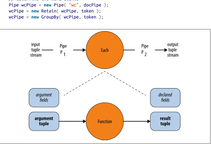
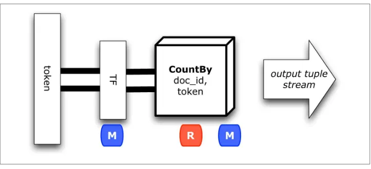
Let’s consider the context of a function within a pipe assembly, as shown in Figure 2-2. At runtime, a pipe assembly takes an input stream of tuples and produces an output stream of tuples.
Figure 2-2. Pipe assembly
Note that by inserting an operation, we must add another pipe. Pipes get connected together in this way to produce pipe assemblies. Looking into this in more detail, as
Figure 2-2 shows, an operation takes an argument tuple—one tuple at a time—and produces a result tuple. Each argument tuple from the input stream must fit the argu‐ ment fields defined in the operation class. Similarly, each result tuple going to the output stream must fit the declared fields.
Now let’s place this new class into a ScrubFunction.java source file. Then we need to change the docPipe pipe assembly to insert our custom operation immediately after the tokenizer:
Fields scrubArguments = new Fields( "doc_id", "token" );
ScrubFunction scrubFunc = new ScrubFunction( scrubArguments );
docPipe = new Each( docPipe, scrubArguments, scrubFunc, Fields.RESULTS );
Notice how the doc_id and token fields are defined in the scrubArguments parameter. That matches what we specified in the constructor. Also, note how the Each operator uses Field.RESULTS as its field selector. In other words, this tells the pipe to discard argument tuple values (from the input stream) and instead use only the result tuple values (for the output stream).
Figure 2-3 shows how an Each operator inserts a Function into a pipe. In this case, the new customized ScrubFunction is fitted between two pipes, both of which are named
docPipe. That’s another important point: pipes have names, and they inherit names
from where they connect—until something changes, such as a join. The name stays the same up until just before the GroupBy aggregation:
// determine the word counts
PipewcPipe = new Pipe( "wc", docPipe );
wcPipe = new Retain( wcPipe, token );
wcPipe = new GroupBy( wcPipe, token );
Figure 2-3. Each with a function
Then we create a new pipe named wc and add a Retain subassembly. This discards all the fields in the tuple stream except for token, to help make the final output simpler. We put that just before the GroupBy to reduce the amount of work required in the aggregation.
Look in the part3/src/main/java/impatient/ directory, where the Main.java and Scrub‐ Function.java source files have already been modified. You should be good to go.
To build:
$ gradle clean jar
To run:
$ rm -rf output
$ hadoop jar ./build/libs/impatient.jar data/rain.txt output/wc
$ more output/wc/part-00000
A gist on GitHub shows building and running “Example 3: Customized Operations”. If your run looks terribly different, something is probably not set up correctly. Ask the developer community for advice.
Scrubbing Tokens
Previously in “Example 2: The Ubiquitous Word Count” we used a RegexSplitGenera‐ tor to tokenize the text. That built-in operation works quite well for many use cases.
“Example 3: Customized Operations” used a custom operation in Cascading to “scrub” the token stream prior to counting the tokens. It’s important to understand the trade-offs between these two approaches. When should you leverage the existing API, versus extending it?
One thing you’ll find in working with almost any text analytics at scale is that there are lots of edge cases. Cleaning up edge cases—character sets, inconsistent hyphens, dif‐ ferent kinds of quotes, exponents, etc.—is usually the bulk of engineering work. If you try to incorporate every possible variation into a regex, you end up with code that is both brittle and difficult to understand, especially when you hit another rare condition six months later and must go back and reread your (long-forgotten) complex regex notation.
Identifying edge cases for text analytics at scale is an iterative process, based on learnings over time, based on experiences with the data. Some edge cases might be encountered only after processing orders of magnitude more data than the initial test cases. Also, each application tends to have its own nuances. That makes it difficult to use “off the shelf ” libraries for text processing in large-scale production.
So in “Example 3: Customized Operations” we showed how to extend Cascading by subclassing BaseOperation to write our own “scrubber.” One benefit is that we can handle many edge cases, adding more as they become identified. Better yet, in terms of separation of concerns, we can add new edge cases as unit tests for our custom class, then code to them. More about unit tests later.
For now, a key point is that customized operations in Cascading are not user-defined functions (UDFs). Customized operations get defined in the same language as the rest of the app, so the compiler is aware of all code being added. This extends the Cascading API by subclassing, so that the API contract must still be honored. Several benefits apply —which are the flip side of what a programmer encounters in Hive or Pig apps, where integration occurs outside the language of the app.
Operations act on the data to transform the tuple stream, filter it, analyze it, etc. Think about the roles that command-line utilities such as grep or awk perform in Linux shell scripts—instead of having to rewrite custom programs.
Similarly, Cascading provides a rich library of standard operations to codify the business logic of transforming Big Data. It’s relatively simple to develop your own custom oper‐ ations, as our text “scrubbing” in “Example 3: Customized Operations” shows. However, if you find yourself starting to develop lots of custom operations every time you begin to write a Cascading app, that’s an anti-pattern. In other words, it’s a good indication that you should step back and reevaluate.
What is the risk in customizing the API components? That goes back to the notion of pattern language. On one hand, the standard operations in Cascading have been de‐ veloped over a period of years. They tend to cover a large class of MapReduce applica‐ tions already. The standard operations encapsulate best practices and design patterns for parallelism. On the other hand, if you aren’t careful while defining a custom oper‐ ation, you may inadvertently introduce a performance bottleneck. Something to think about.
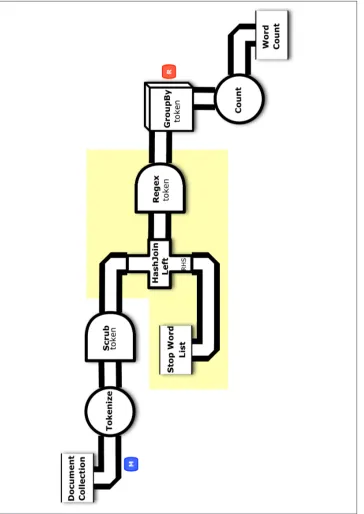
Example 4: Replicated Joins
Figure 2-4. Conceptual flow diagram for “Example 4: Replicated Joins”
Starting from the source code directory that you cloned in Git, connect into the part4
subdirectory. First let’s add another source tap to read the stop words list as an input data set:
String stopPath = args[ 2 ];
Fields stop = new Fields( "stop" );
Tap stopTap = new Hfs( new TextDelimited( stop, true, "\t" ), stopPath );
Next we’ll insert another pipe into the assembly to connect to the stop words source tap. Note that a join combines data from two or more pipes based on common field values. We call the pipes streaming into a join its branches. For the join in our example, the existing docPipe provides one branch, while the new stopPipe provides the other. Then we use a HashJoin to perform a left join:
// perform a left join to remove stop words, discarding the rows // which joined with stop words, i.e., were non-null after left join
PipestopPipe = new Pipe( "stop" );
PipetokenPipe = new HashJoin( docPipe, token, stopPipe, stop, new LeftJoin() );
When the values of the token and stop fields match, the result tuple has a non-null value for stop. Then a stop word has been identified in the token stream. So next we discard all the non-null results from the left join, using a RegexFilter:
tokenPipe = new Each( tokenPipe, stop, new RegexFilter( "^$" ) );
Tuples that match the given pattern are kept, and tuples that do not match get discarded. Therefore the stop words all get removed by using a left join with a filter. This new
tokenPipe can be fitted back into the wcPipe pipe assembly that we had in earlier ex‐ amples. The workflow continues on much the same from that point:
Pipe wcPipe = new Pipe( "wc", tokenPipe );
Last, we include the additional source tap to the FlowDef:
// connect the taps, pipes, etc., into a flow
FlowDef flowDef = FlowDef.flowDef() .setName( "wc" )
.addSource( docPipe, docTap ) .addSource( stopPipe, stopTap ) .addTailSink( wcPipe, wcTap );
Modify the Main method for these changes. This code is already in the part4/src/main/ java/impatient/ directory, in the Main.java file. You should be good to go.
To build:
$ gradle clean jar
To run:
$ rm -rf output
Again, this uses the same input from “Example 1: Simplest Possible App in Cascad‐ ing”, but now we expect all stop words to be removed from the output stream. Common words such as a, an, as, etc., have been filtered out.
You can verify the entire output text in the output/wc partition file, where the first 10 lines (including the header) should look like this:
$ head output/wc/part-00000
The flow diagram will be in the dot/ subdirectory after the app runs. For those keeping score, the resulting physical plan in Apache Hadoop uses one map and one reduce.
Again, a GitHub gist shows building and running this example. If your run looks terribly different, something is probably not set up correctly. Ask the developer community for advice.
Stop Words and Replicated Joins
Let’s consider why we would want to use a stop words list. This approach originated in work by Hans Peter Luhn at IBM Research, during the dawn of computing. The reasons for it are twofold. On one hand, consider that the most common words in any given natural language are generally not useful for text analytics. For example, in English, words such as “and,” “of,” and “the” are probably not what you want to search and probably not interesting for Word Count metrics. They represent high frequency and low semantic value within the token distribution. They also represent the bulk of the processing required. Natural languages tend to have on the order of 105 words, so the
potential size of any stop words list is nicely bounded. Filtering those high-frequency words out of the token stream dramatically reduces the amount of processing required later in the workflow.
On the other hand, you may also want to remove some words explicitly from the token stream. This almost always comes up in practice, especially when working with public discussions such as social network comments.
Think about it: what are some of the most common words posted online in comments? Words that are not the most common words in “polite” English? Do you really want those words to bubble up in your text analytics? In automated systems that leverage
unsupervised learning, this can lead to highly embarrassing situations. Caveat machi‐ nator.
Next, let’s consider working with a Joiner in Cascading. We have two pipes: one for the “scrubbed” token stream and another for the stop words list. We want to filter all in‐ stances of tokens from the stop words list out of the token stream. If we weren’t working in MapReduce, a naive approach would be to load the stop words list into a hashtable, then iterate through our token stream to lookup each token in the hashtable and delete it if found. If we were coding in Hadoop directly, a less naive approach would be to put the stop words list into the distributed cache and have a job step that loads it during setup, then rinse/lather/repeat from the naive coding approach described earlier.
Instead we leverage the workflow orchestration in Cascading. One might write a custom operation, as we did in the previous example—e.g., a custom Filter that performs look‐ ups on a list of stop words. That’s extra work, and not particularly efficient in parallel anyway.
Cascading provides for joins on pipes, and conceptually a left outer join solves our requirement to filter stop words. Think of joining the token stream with the stop words list. When the result is non-null, the join has identified a stop word. Discard it.
Understand that there’s a big problem with using joins at scale in Hadoop. Outside of the context of a relational database, arbitrary joins do not perform well. Suppose you have N items in one tuple stream and M items in another and want to join them? In the general case, for an arbitrary join, that requires N × M operations and also introduces a data dependency, such that the join cannot be performed in parallel. If both N and M
are relatively large, say in the millions of tuples, then we’d end up processing 1012
operations on a single processor—which defeats the purpose in terms of leveraging MapReduce.
Keep in mind that stop words lists tend to be bounded at approximately 105 keywords.
That is relatively sparse when compared with an arbitrarily large token stream. At typical “web scale,” text analytics use cases may be processing billions of tokens, i.e., several orders of magnitude larger than our largest possible stop words list. Sounds like a great use case for HashJoin.
Comparing with Apache Pig
When it comes to the subject of building workflows—specifically about other abstrac‐ tions on top of Hadoop—perhaps the most frequent question about Cascading is how it compares with Apache Hive and Apache Pig. Let’s take a look at comparable imple‐ mentations of the “Example 4: Replicated Joins” app in both Pig and Hive.
First you’ll need to install Pig according to the documentation, in particular the “Getting Started” chapter. Unpack the download and set the PIG_HOME and PIG_CLASSPATH en‐ vironment variables. Be sure to include Pig in your PATH environment variable as well.
Starting from the source code directory that you cloned in Git, connect into the part4
subdirectory. The file src/scripts/wc.pig shows source for an Apache Pig script that im‐ plements Word Count:
docPipe = LOAD '$docPath' USING PigStorage('\t', 'tagsource') AS (doc_id, text);
docPipe = FILTER docPipe BY doc_id != 'doc_id';
stopPipe = LOAD '$stopPath' USING PigStorage('\t', 'tagsource') AS (stop:chararray);
stopPipe = FILTER stopPipe BY stop != 'stop';
-- specify a regex operation to split the "document" text lines into a token stream
tokenPipe = FOREACH docPipe
GENERATE doc_id, FLATTEN(TOKENIZE(LOWER(text), ' [](),.')) AS token;
tokenPipe = FILTER tokenPipe BY token MATCHES '\\w.*';
-- perform a left join to remove stop words, discarding the rows -- which joined with stop words, i.e., were non-null after left join
tokenPipe = JOIN tokenPipe BY token LEFT, stopPipe BY stop;
tokenPipe = FILTER tokenPipe BY stopPipe::stop IS NULL;
-- determine the word counts
tokenGroups = GROUP tokenPipe BY token;
wcPipe = FOREACH tokenGroups
GENERATE group AS token, COUNT(tokenPipe) AS count;
-- output
STORE wcPipe INTO '$wcPath' using PigStorage('\t', 'tagsource'); EXPLAIN -out dot/wc_pig.dot -dot wcPipe;
To run the Pig app:
$ rm -rf output $ mkdir -p dot