www.elsevier.com/locate/dsw
A parallel primal–dual simplex algorithm
Diego Klabjan
∗, Ellis L. Johnson, George L. Nemhauser
School of Industrial and Systems Engineering, Georgia Institute of Technology, Atlanta, GA 30332-0205, USA
Received 1 June 1999; received in revised form 1 December 1999
Abstract
Recently, the primal–dual simplex method has been used to solve linear programs with a large number of columns. We present a parallel primal–dual simplex algorithm that is capable of solving linear programs with at least an order of magnitude more columns than the previous work. The algorithm repeatedly solves several linear programs in parallel and combines the dual solutions to obtain a new dual feasible solution. The primal part of the algorithm involves a new randomized pricing strategy. We tested the algorithm on instances with thousands of rows and tens of millions of columns. For example, an instance with 1700 rows and 45 million columns was solved in about 2 h on 12 processors. c2000 Elsevier Science B.V. All rights reserved.
Keywords:Programming=linear=algorithms; Large-scale systems
1. Introduction
This paper presents a parallel primal–dual simplex algorithm that is capable of solving linear programs with thousands of rows and millions of columns. For example, an instance with 1700 rows and 45 million columns was solved in about 2 h on 12 processors. The largest instance we solved has 25 000 rows and 30 mil-lion columns. Such linear programs arise, for example, in airline crew scheduling and several other applica-tions as relaxaapplica-tions of set partitioning problems [4].
∗Correspondence address: Department of Mechanical and
In-dustrial Engineering, University of Illinois at Urbana-Champaign, Urbana, IL 61801, USA.
E-mail addresses: [email protected] (D. Klabjan), ellis. [email protected] (E.L. Johnson), nemhauser@isye. gatech.edu (G.L. Nemhauser).
Primal–dual algorithms appear to have originated with Dantzig et al. [9] and have been applied to many combinatorial problems such as network ows Ahuja et al. [1] and matching, Edmonds [10]. Recently, Hu [11] and Hu and Johnson [12] have developed a primal–dual simplex algorithm that is designed to solve LPs with a very large number of columns. The primal–dual simplex iterates between solving primal subproblems over a restricted number of columns and dual steps. In this paper, we parallelize the dual step of the Hu-Johnson algorithm and obtain signicant speedups. Since the number of dual steps is small, information is passed infrequently, so it is ecient to partition the columns among several computers, i.e. to use a distributed memory system.
Bixby and Martin [7] present a dual simplex algo-rithm with parallel pricing. However, their approach requires a shared memory system to achieve good
speedups since pricing is done over all columns after every simplex iteration. Bixby and Martin cite other literature on parallel simplex algorithms, none of which is related to our work.
In Section 2, we review the primal–dual algorithm. Section 3 presents the parallel primal–dual algorithm. Section 4 gives the computation results.
2. Primal–dual algorithm
We consider the LP
min{cx:Ax=b; x¿0}; (P)
whereA∈Qn×m; b ∈Qm; x ∈Qn andQk is the set ofk-dimensional rational numbers.
The dual is
max{b:A6c}: (D)
The primal–dual algorithm is ecient only if the number of columns is much larger than the number of rows, so we assume thatn≫m.
A primal subproblem is a problem with only a sub-set of columns from the constraint matrixAand cor-responding objective coecients. The reduced cost of columnjwith respect to a dual vectorisrc
j =cj−
Aj, whereAjis thejth column ofA.
We start with a statement of the primal–dual algo-rithm 1 from Hu [11].
The algorithm maintains a dual feasible solution. At each iteration the algorithm produces a dual vector
which is not necessarily dual feasible. The two dual vectors are then combined into a new dual feasible vector that gives the largest improvement to the dual objective. The dual vector is used to select columns for the next primal subproblem. The procedure is then iterated.
3. Parallel primal–dual algorithm
3.1. Algorithm
The key idea of parallelization is to form several primal subproblems that are solved in parallel. The new dual feasible vector is a convex combination of optimal dual vectors arising from the subproblems and the current dual feasible solution. This can be seen as a
natural way of parallelizing the primal–dual algorithm since each successive is a convex combination of the initialand all previouss.
Algorithm 1. The primal–dual algorithm
1. A dual feasible solution and a primal feasible subproblem are given.
2. Solve the subproblem and let be a dual optimal solution andxa primal optimal solution.
3. Ifb=cx, then (x; ) are optimal solutions. Ifis dual feasible, then (x; ) are optimal solutions. 4. Find an∈Q;0¡ ¡1 such that (1−)+
is dual feasible and is maximum. Set= (1−
)+.
5. Remove all the columns from the subproblem ex-cept the basic ones. Add a set of columns with the lowest reduced costs rc
j to form a new subprob-lem.
6. Go to step 2.
Suppose we havepprocessors and each column of
A is assigned with equal probability to a processor. A detailed description of the parallel primal–dual algorithm 2 follows.
Algorithm 2. The parallel primal–dual algorithm
1. A dual feasible solutionandpprimal feasible subproblemsPi; i= 1; : : : ; pare given.
2. fori= 1 topin parallel do
3. Solve the subproblemPiand letibe a dual op-timal solution andxia primal optimal solution. 4. Ifb=cxi, then (xi; ) are optimal solutions. 5. end for
6. Find∈Qp+;Pp
i=1 i61 such that
˜
= 1−
p X
i=1
i !
+
p X
i=1
ii (1)
is dual feasible andb˜is maximum. Set= ˜. 7. If b=cxi for some i, then (xi; ) are optimal
solutions.
8. fori= 1 topin parallel do
9. Remove all the columns from the subproblem
Piexcept the basic columns. Usingand cont-rolled randomization append new columns toPi. 10. end for
11. Go to step 3.
Forming initial subproblems(Step 1): Since it is expensive to compute the reduced costs of a large number of columns, unless the initial dual solution
is thought to be ‘good’, we choose columns for the ini-tial subproblems randomly. We add articial variables with big costs to each subproblem to make them pri-mal feasible. Once an articial variable becomes non-basic, we remove it permanently from the subproblem (step 3, or step 9 if the internal functionalities of the linear programming solver are not available).
On the other hand, if the initialis thought to be ‘good’, then the controlled randomization procedure (step 9) described below is applied.
Combining dual solutions (Step6): In step 6 we nd a convex combination of vectors; 1; : : : ; pthat yields a dual feasible vector and gives the largest in-crease in the dual objective value. Let v=b and
vi=bi; i= 1; : : : ; p. Note thatvi¿vfor alliby weak duality. The dual feasibility constraints
1−
can be rewritten as p
X
i=1
i(rc−rci)6rc:
Hencecan be obtained by solving the LP
max
This is an LP withpvariables andn+1 constraints, wherepis very small andnis very large. Its dual is
minz+
We solve (3) with a SPRINT approach due to Forrest, see [2,6]. We start with a subproblem con-sisting of the z column and some randomly chosen
ycolumns. Then we iterate the following steps. Let
be an optimal dual vector. Delete all the columns from the subproblem except the basic columns and thez column. Add to the current subproblem a sub-set of columns of (3) with the smallest reduced cost based on, and then solve it. If all the columns have nonnegative reduced cost, then the solution is optimal. If we compute reduced costs for (3) directly from the constraints in (2), then for a single column we would have to computepreduced costs for a column in P, one for each i, and then compute their sum weighted with the dual vector of (3). Instead, we can compute the reduced costrcj more eciently by rewriting
Hence at each iteration of SPRINT, before forming the new subproblem, we rst compute ˜and then the pricing for (3) is equivalent to the pricing for P with respect to ˜.
We now show that the stopping criteria in step 7 is also implied by the dual feasibility of the’s. Note that the dual feasibility check could be also done after step 5 but that would be very costly to perform because of the huge number of columns.
Proposition 1. IfPpj=1 j= 1is an optimal solution to(2); then there is an i such thatb=cxi.Ifi is dual feasible;thenb=cxi.
Pp
j=1 j(vj−v) = 0. Sincevj−v¿0 by weak duality andj¿0, it follows thatj(vj−v) = 0 for allj. Since there is anisuch thati¿0,v=vi.
Ifiis dual feasible, theni= 1 andj= 0 for all
j6=iis feasible to (2) and optimal by weak duality. Hencev=vi.
Choosing columns for the subproblems(Step9): In addition to needing columns with low reduced cost, it is important that subproblems receive a representative sample of columns from the original problem. This is achieved by a controlled randomization process based on the current dual solution.
The following parameters are used in assigning columns.
nSub: the expected number of columns given to a subproblem (this is determined empirically);
nSubLow: the number of common low reduced cost
columns given to each subproblem in Case 1 below (to be discussed later in the section);
nSub0: the number of columnsjwithrc j = 0;
minRC: ifnSub0¡ nSubLow, thenminRC ¿0 is a
number such that the number of columns with reduced cost less thanminRCisnSubLow;
maxRC: ifrcj¿ maxRC, then columnjis not con-sidered as a candidate for a subproblem;
nSubHigh: the number of columns j with rc
j6
maxRC.
To compute maxRC, rst note that we need p·
nSubcolumns. Also we know that there arenSubLow
columns with reduced cost below minRC. Thus as-suming at the rst iteration that the columns have been uniformly distributed among the processors, we have
maxRC=p·minRC·nSub
nSubLow :
We compute nSubHighonly at the rst iteration. In subsequent iterations we retain the value ofnSubHigh
and adjustmaxRC accordingly. We consider 3 cases.
Case 1: nSub0¡ nSubLow. All columns j with
rc
j ¡ minRC are given to each subproblem. Every
column j withminRC6rc
j6maxRC is a candidate
for a subproblem. We select columns using the idea that the lower reduced cost columns should have a higher probability of being selected.
Letpjbe the probability that a columnjfrom the initial constraint matrix Ais added to subproblem i.
Since there is no reason to distinguish between problems, the probability does not depend on the sub-problem indexi. Clearlypjshould be a nonincreasing function of the reduced costrc
j and
In order to emphasize the reduced cost we choose the rapidly decreasing function exp(−x2). The value
is determined by
f() =
Becausen is so large, it is too expensive to evaluate
f() or its derivative. Instead, we approximate the value ofusing a ‘bucket’ approach.
Let N be the number of buckets (we use N =
It is easy to derive bounds
ln(PNj=0−1 bj=(nSub−nSubLow))
The function ˜f is continuously dierentiable and decreasing in the interval given by (5). If we use Newton’s method with a starting point in the interval given by (5), the method converges to the solution of the equation ˜f(∗) =nSub−nSubLow(see e.g. [5]). Newton’s method is fast for small values of N and the optimal value∗ is a good approximation to the solution of (4).
Case2:nSub0¿nSubLow; nSub06k·nSub,where
k ¡1 is a parameter (we use k = 1=3). Replace
Case 3: nSub0¿max(nSubLow; k ·nSub). Since there are so many columns withrc
j=0, we assign them randomly to the subproblems. Empirically, we ob-tained good results if the expected number of columns given to each subproblem isnSub=rwhere
r= max
1;nSubHigh
nSub0 ;
nSub02
nSubLow·nSub
:
The remaining columns are assigned by controlled randomization as in Case 1.
Pricing heuristic: It remains to be shown how to eciently nd a reduced cost value such that the num-ber of columns with the reduced cost smaller than that value is a given number k. This is required in both step 9 and the SPRINT algorithm used to solve (3). Using sorting terminology, we want to nd a rankk
element among reduced cost values. Since for our ap-plications we have only an estimate ofk, we want to nd a reduced cost value that yields approximatelyk
columns.
Other approaches are considered in [2,11,6]. Bader and JaJa [3] describe an algorithm for nding a median in parallel, but it is likely to be too slow for our needs since it is targeted to nd exactly the rankkelement. Our approach relies on distributing the columns randomly. Assume that Si is the set of reduced cost values at processori. For simplicity of notation letdj be the reduced cost of columnj(instead ofrc(j:)), i.e.
Si={d1; : : : ; dni}. Our goal is to nd thekth smallest
element in Spi=1Si. For our applicationsk is always much smaller thanni.
The following intuitive observation plays a key role. Let dmi be an element with rank r =⌊k=p⌋ in the
sequenceSiand letd= mini=1; :::; p{dmi}. Letmbe the
number of elements in Spi=1Si that are smaller than
d. Since the numbersdi are randomly distributed, m should be approximately p·r ≈ k. It is clear that
m6p·r. Experiments have shown the validity of the claim. Klabjan [13] gives some theoretical support by proving that r(p−1)6mas ni → ∞ for all i and
k→ ∞.
So the task reduces to nding an element with rank
rinSi. Even here we do not sort the arraySidue to the possible large value ofni. Any exact sequential me-dian nding algorithm is likely to be too slow and too ‘exact’ since we are looking only for an approxima-tion of a rankrelement. Sincek is typically a small number, so isr.
For simplicity we writen; S instead ofni; Si. Lets and ˜r; r6s˜ , be two integers. Suppose that we choose
selements uniformly at random fromSand we denote them asbS. Let ˜dbe the element with rank ˜rinbS. The following theorem forms the basis for our heuristic.
Theorem 1(Klabjan [13]). If all elements in S are dierent;then
E = E(|{di:di6d˜}|) = ˜
r(n+ 1)
s+ 1 :
Since we want the sample sizesto be as small as possible, we choose ˜r= 1. Hences=⌈n=r⌉. For our instancesnranged in millions andrwas always bigger than 500. For example, ifr= 500 andn= 2×10⁶, the sampling size is 40 000.
Note that in step 9 of the parallel primal–dual al-gorithm, we have to nd elements of ranknSubLow andnSubHigh. We need to obtain samples just once since we can use them for both computations.
3.2. Finite convergence
We prove the convergence of the algorithm under the assumption of primal nondegeneracy.
Theorem 2. If problem P is primal nondegenerate and at each iteration all the0reduced cost columns based on are added to each subproblem; then the parallel primal–dual algorithm terminates nitely.
Proof. Suppose the algorithm is in thekth major iter-ation after step 7. Denote byvk
i the optimal value of subproblemi. Consider the LP (2) and its dual, and let (; z; y) be optimal solutions. Since the stopping cri-teria in steps 4 and 7 are not satised, by Proposition 1,Ppi=1i¡1 andv=b ¡ vikfor alli= 1; : : : ; p.
Suppose that=0. Sincev ¡ vik, this is the only fea-sible solution to (2). Therefore,conv{; 1; : : : ; p}is the singleton, implying that=ifor alli=1; : : : ; p. Since1=is dual feasible and by Proposition 1, the
stopping criteria in step 7 is fullled, there is a con-tradiction. Thus6= 0 and the optimal value to (3) is positive.
Since Ppi=1i¡1, by complementary slackness
z= 0. The optimal value to (3) is positive and hence Pnj=1rc
jyj¿0. Since rcjyj¿0 for all
yj0¿0 and rcj0¿0. By complementary slackness Pp
i=1i(rcj0 −rc i
j0) =rcj0. Since Pp
i=1i¡1 and
rc
j0¿0, it easily follows that there is an index
i0;16i06psuch thatrc
i0 j0 ¡0.
Consider now the columnj0 of P. Since in (2) the
rowj0 is at equality, it follows thatrcj0˜ = 0. By as-sumption the column is appended to each subproblem, hence to the subproblemi0. By the nondegeneracy
as-sumption it follows thatvki0+1¡ vk i0. Considerok=
Pp
i=1vik. Sincevik¿vki+1for alli= 1; : : : ; p andvk
i0¿ vki0+1, it follows thatok¿ ok+1 for
allk. Since there are only nitely many subproblems, the number of dierent values ofvk
i for alli= 1; : : : ; p andkis nite. The claim now follows due to the nite number of dierent values in theosequence and the monotonicity propertyok¿ ok+1.
Note that the dual objective value increases at each iteration regardless of degeneracy, however the nite-ness argument does not follow from the nondegener-acy assumption.
4. Computational experiments
4.1. Computing environment
All computational experiments were performed on a cluster of machines comprised of 48 300 MHz Intel Dual Pentium IIs, resulting in 96 processors available for parallel program execution. All ma-chines are linked via 100 MB point-to-point Ethernet switched via a Cisco 5500 network switch. Each node has 512 MBytes of main memory.
The operating system used was Sun Solaris x86, version 2.5.1, which oers facilities for parallel com-puting like remote shell (rsh commands), global le system support via NFS, and parallel computing libraries like MPI or PVM. The cluster is represen-tative of typical machines of this type, in its rela-tively slow internode communications and its good cost=performance ratio vs. specialized parallel ma-chines like the CM-5, the Intel Paragon, or the IBM SP-2 machines.
The parallel implementation uses the MPI mes-sage passing interface MPI, MPICH implementation version 1.0, developed at Argonne National Labs.
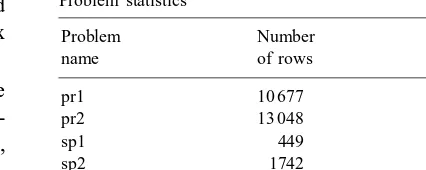
Table 1 Problem statistics
Problem Number Number
name of rows of columns
pr1 10 677 17 045 897
pr2 13 048 9 234 109
sp1 449 42 134 546
sp2 1742 45 952 785
sp3 3143 46 546 240
The MPI message passing standard is widely used in the parallel computing community. It oers facilities for creating parallel programs to run across cluster machines and for exchanging information between processes using message passing procedures like broadcast, send, receive and others.
The linear programming solver used was CPLEX, CPLEX, Optimization [8], version 5.0.
4.2. Problem instances
The instances are listed in Table 1. The set parti-tioning instances sp1, sp2, and sp3 are airline crew scheduling problems (see e.g. [13]). All of these instances may contain some duplicate columns but, because of the method of generation, no more than approximately 5% of the columns are dupli-cates. For this reason we do not remove duplicate columns.
The remaining two instances also are from Klabjan [13]. The problems have a substantial set partitioning portion. They occurred in a new approach to solving the airline crew scheduling problem. The pr2 problem is particularly hard due to the high number of rows and primal degeneracy.
All instances have on average 10 nonzeros per column.
4.3. Implementation and parameters
Because some problems are highly primal de-generate, the primal LP solver struggles to make progress. Therefore, we globally perturb the right hand side and then we gradually decrease the per-turbation. Precisely, we perturb a row Aix=bi of P to a ranged row bi −16Aix6bi +2, where
to nd an optimal solution to the perturbed prob-lem, so we apply the parallel primal–dual method until
mini=1; :::; p{vi} −v mini=1; :::; p{vi}
¿gap;
wheregap is a constant. The gap is checked at step 7 of the algorithm. If gap is belowgap, then the per-turbation is reduced by a factor of 2, i.e. each 1; 2
becomes 1=2; 2=2. Once all of the epsilons drop
below 10−6, the perturbation is removed entirely.
For our experiments we setgap= 0:03.
For set partitioning problems a starting dual fea-sible vector is = 0 if all the cost coecients are nonnegative. However there are many columns with 0 cost resulting in many columns with 0 reduced cost. Hence, we perturbby componentwise subtracting a small random number. This decreases the initial dual objective but the newis not ‘jammed’ in a corner. For instances pr1 and pr2 we use the same idea, how-everneeds to be changed to accommodate the extra rows and variables (see [13]).
At the rst iteration we do not usually have a warm start and we found that the dual simplex is much faster than the primal simplex. However, a warm start is available at each successive iteration since we keep the optimal basis from the previous iteration. Hence the primal simplex is applied.
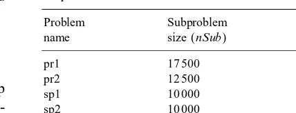
Next we discuss the parameters nSub and nSubLow. Empirically, we found that nSubLow=
nSub=2:5 works best. We use this relationship in all of our experiments. Table 2 givesnSubfor the paral-lel primal–dual algorithm and the number of columns used in the sequential version of the code. In each case the parameters have been determined empirically to be the subproblem sizes that have given the best result. They will be discussed further in Section 4.4.
Finally, we observed empirically that for some in-stances (sp1 and sp2) and at certain iterations the al-gorithm spends too much time solving subproblems. So we impose an upper bound of 30 min on the exe-cution time of subproblems. This improves the overall execution time. Note that quitting the optimization be-fore reaching the optimality of subproblems does not aect the correctness of the algorithm.
We start SPRINT for solving (3) with 40 000 ran-dom columns and in each successive iteration we append 50 000 best reduced cost columns. Typically
Table 2 Subproblem sizes
Problem Subproblem Subproblem
name size (nSub) size, seq.
pr1 17 500 30 000
pr2 12 500 30 000
sp1 10 000 10 000
sp2 10 000 35 000
sp3 5 000 10 000
three iterations of SPRINT are required, the third one just conrming optimality. The execution time never exceeded 1 min.
4.4. Results
Due to the large number of columns and a main memory of 512 MBytes, we were not able to solve any problem on a single machine. We implemented a variant of the sequential primal–dual algorithm in which the columns are distributed across the ma-chines. Only the pricing is carried out in parallel. We call it the primal–dual algorithm with parallel pricing. In essence, a true sequential primal–dual al-gorithm would dier only in pricing all the columns sequentially. Based on the assumption that pricing is a linear time task (which is the case for our pricing procedure), we estimated the execution times of a true sequential primal–dual implementation.
The gain of the parallelization of the primal–dual algorithm is twofold; one is the parallel pricing strat-egy, and the second is having multiple subproblems. The rst one is addressed by the primal–dual algo-rithm with parallel pricing. We give the speedups in Table 3. As we can see the parallel pricing heuristic has a big impact when the overall execution time is small and the number of columns is big, i.e. the sp1 problem. For the remaining problems the parallel pric-ing does not have a dominant eect.
Table 3
Eect of parallel pricing
Problem Number of Execution
name processors time (s)
pr1 1 19 200
8 17 140
pr2 1 81 000
8 76 860
sp1 1 3 000
8 1 100
sp2 1 24 000
8 10 320
sp3 1 62 460
8 50 160
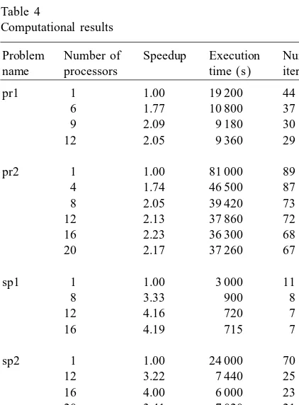
Table 4
Computational results
Problem Number of Speedup Execution Number of name processors time (s) iterations
pr1 1 1.00 19 200 44
6 1.77 10 800 37
9 2.09 9 180 30
12 2.05 9 360 29
pr2 1 1.00 81 000 89
4 1.74 46 500 87
8 2.05 39 420 73
12 2.13 37 860 72
16 2.23 36 300 68
20 2.17 37 260 67
sp1 1 1.00 3 000 11
8 3.33 900 8
12 4.16 720 7
16 4.19 715 7
sp2 1 1.00 24 000 70
12 3.22 7 440 25
16 4.00 6 000 23
20 3.41 7 020 21
sp3 1 1.00 62 460 62
12 2.30 27 120 57
16 2.50 24 960 53
20 2.51 24 840 50
So our main conclusion is that the speedups are sig-nicant when the number of processors is between 4 and 12. The execution times can be improved even
Table 5
The breakdown of execution times on 12 processors
Problem Total Step 3 Steps 6,7 Step 9
name time time time time
pr1 9 360 5 183 2727 1150
pr2 37 860 32 689 3166 1005
sp1 720 127 190 251
sp2 7 440 3 823 689 1700
sp3 27 120 19 425 1 887 3420
further by using a pure shared memory machine. On average the communication time was 45 s per itera-tion. A shared memory computing model would def-initely lead to improvements for the sp1 problem. Additional improvement in the execution time of the sp1 problem might result by allowingto be ‘slightly’ infeasible. When solving LP (3), we could perform just two SPRINT iterations and then quit without prov-ing optimality.
A breakdown of execution times is shown in Table 5. For the harder problems (pr1, pr2 and sp3) more than 70% of the time is spent in solving the subprob-lems, however for the sp1 problem only 17% of the time is spent on subproblem solving. A better com-munication network would improve the times for step 9, but for the harder problems it would not have a sig-nicant impact.
Although we use the same subproblem size regard-less of the number of processors in our experiments reported in Table 4, the subproblem size should de-pend on the number of processors. The smaller the number of processors, the bigger the subproblem size should be. For a large number of processors, solv-ing many small subproblems is better than spendsolv-ing time on solving larger subproblems. For the pr1 prob-lem the optimal subprobprob-lem sizes are 30 000, 25 000, 17 500 forp= 6;9;12, respectively.
The largest problem we have solved so far has 30 million columns and 25 000 rows [13]. The execution time on 12 processors was 30 h.
There are several open questions regarding an ef-cient implementation of a parallel primal–dual sim-plex algorithm. Subproblem size is a key question and the development of an adaptive strategy could lead to substantial improvements. To make subproblems even more dierent, columns with negative reduced cost based on i can be added to the subproblems. We made an initial attempt in this direction but more experimentation needs to be done.
Acknowledgements
This work was supported by NSF grant DMI-9700285 and United Airlines, who also provided data for the computational experiments. Intel Corpora-tion funded the parallel computing environment and ILOG provided the linear programming solver used in computational experiments.
References
[1] R. Ahuja, T. Magnanti, J. Orlin, Network Flows, Prentice-Hall, Englewood Clis, NJ, 1993.
[2] R. Anbil, E. Johnson, R. Tanga, A global approach to crew pairing optimization, IBM Systems J. 31 (1992) 71–78.
[3] D. Bader, J. JaJa, Practical parallel algorithms for dynamic data redistribution, median nding, and selection, Proceedings of the 10th International Parallel Processing Symposium, 1996.
[4] C. Barnhart, E. Johnson, G. Nemhauser, N. Savelsbergh, P. Vance, Branch-and-price: column generation for solving huge integer programs, Oper. Res. 46 (1998) 316–329.
[5] D. Bertsekas, Nonlinear Programming, Athena Scientic, Belmont, MA 1995, pp. 79 –90.
[6] R. Bixby, J. Gregory, I. Lustig, R. Marsten, D. Shanno, Very large-scale linear programming: a case study in combining interior point and simplex methods, Oper. Res. 40 (1992) 885–897.
[7] R. Bixby, A. Martin, Parallelizing the dual simplex method, Technical Report CRPC-TR95706, Rice University, 1995. [8] CPLEX Optimization, Using the CPLEX Callable Library,
5.0 Edition, ILOG Inc., 1997.
[9] G. Dantzig, L. Ford, D. Fulkerson, A primal–dual algorithm for linear programs, in: H. Kuhn, A. Tucker (Eds.), Linear Inequalities and Related Systems, Princeton University Press, Princeton, NJ, 1956, pp. 171–181.
[10] J. Edmonds, Maximum matching and a polyhedron with 0-1 vertices, J. Res. Nat. Bur. Standards 69B (1965) 125–130. [11] J. Hu, Solving linear programs using primal–dual
subproblem simplex method and quasi-explicit matrices, Ph.D. Dissertation, Georgia Institute of Technology, 1996. [12] J. Hu, E. Johnson, Computational results with a primal–dual
subproblem simplex method, Oper. Res. Lett. 25 (1999) 149– 158.