arXiv:1709.05492v1 [quant-ph] 16 Sep 2017
Nasim Shahmansoori,1 Farhad Taher Ghahramani,2 and Afshin Shafiee1, 2,∗
1
Research Group On Foundations of Quantum Theory and Information,
Department of Chemistry, Sharif University of Technology, P.O.Box 11365-9516, Tehran, Iran
2
Foundations of Physics Group, School of Physics,
Institute for Research in Fundamental Sciences (IPM), P.O. Box 19395-5531, Tehran, Iran
In this study, we examine the dynamics of a macroscopic quantum system in interaction with a non-equilibrium environment. The system is conveniently described as a particle confined in a double-well potential. The environment is composed of two independent equilibrium environments at different temperatures. We use the time-dependent perturbation theory to describe the dynamics without any explicit Born and Markov assumptions. We demonstrate that in two environments at same temperatures the short-time dynamics is affected by the interference between two environments through the system. In the non-equilibrium environment, the quantum coherence of the system essentially has an oscillatory dependence on the temperature difference between two environments. Nonetheless, for a wide range of temperature differences, the non-equilibrium environment enhances the quantum coherence. This effect is weakened by the force the macroscopic system exerts on environmental particles.
Keywords: Macroscopic Quantum Systems, Non-equilibrium Environment, Decoherence Theory
1. INTRODUCTION
Quantum coherence is the distinguishing feature of isolated microscopic systems. In macroscopic systems, however, it is destroyed due to the inevitable interaction between the system and the surrounding environment, a phenomenon called decoherence [1, 2]. This interaction brings out some novel physics, such as lasing without inversion or extracting work from a single heat bath [3–6]. In the theory of open quantum systems, it is usually assumed that the environment is in thermal equilibrium [7, 8]. Such an assumption not only faithfully projects most environments but also greatly simplifies theoretical analysis. Nonetheless, there are physical and especially biological situations where the environ-ment is not in thermal equilibrium. In these cases, the environenviron-ment has the opportunity to influence the quantum evolution in a manner that is more rich and complex than simply acting to randomize relative phases and dissipate energy. Light-induced ultra-fast coherent electronic processes in chemical and biological systems, superconducting circuits and quantum dots are examples where non-equilibrium effects are important [9–14].
The dynamics of quantum systems in non-equilibrium environments has been studied in a number of contexts. Myatt and co-workers studied the decoherence of trapped ions coupled to engineered reservoirs, where the internal state and the coupling strength can be controlled [15]. Schriefl and co-workers studied the dephasing of a two-level system, coupled to non-stationary noise modeling interacting defects [16] and to non-stationary classical intermittent noise [17]. Kohler and Sols reported the emergence of recoherence in the dissipative dynamics of a harmonic oscillator, coupled linearly through its position and momentum to two independent heat baths at the same temperatures [18]. Gordon and co-workers discussed the control of quantum coherence and the inhibition of dephasing using stochastic control fields [19]. Clausen and co-workers demonstrated a bath-optimized minimal energy control scheme to use arbitrary time-dependent perturbations to slow decoherence of quantum systems interacting with non-Markovian but stationary environments [20]. The well-known increase of the decoherence rate with the temperature, for a quantum system coupled to a linear thermal bath, no longer holds for a different bath dynamics. This is shown by means of a simple classical nonlinear bath [21]. Emary considered two examples of nonlinear baths weakly coupled to a quantum system and showed that the decoherence rate is a monotonic decreasing function of temperature [22]. Beer and Lutz discussed decoherence in a general non-equilibrium environment consisting of several equilibrium baths at different temperatures, described as a single effective bath with a time-dependent temperature [23]. Martens studied the non-equilibrium response of the environment by a non-stationary random function which offers the possibility of the control of quantum decoherence by the detailed properties of the environment [24]. Li and co-workers concluded that the amount of the steady quantum coherence increases with the temperature difference of the two heat baths coupled to a three-state system [25]. If two heat baths have the same temperature, all quantum coherence vanishes and the dynamics returns to the equilibrium case. Moreno and co-workers showed that nested environments can improve coherence of a central system as the coupling between near and far environment increases [26].
Non-equilibrium quantum dynamics is also attractive from fundamental point of view. Ludwig and co-workers showed that there is an optimal dissipation strength for which the entanglement between two coupled oscillators in-teracting with a non-equilibrium environment is maximized [27]. Castillo and co-workers demonstrated that under non-equilibrium thermal conditions, in a certain range of temperature gradients, Leggett-Garg inequality violation can be enhanced [28]. In all such studies,in principle, the possibility of controlling decoherence is of great importance.
dynamics of the macroscopic system, especially the phenomenon of macroscopic quantum tunneling, can be studied in the typical double-well potential. At sufficiently low temperatures, the system’s Hamiltonian can be expanded by two first states of energy. When the two-level system couples linearly to an oscillator environment, the result is the renowned Spin-Boson model [7, 32]. Due to decoherence, then, a mixture of localized states of the system appears.
Here, we examine the effective dynamics of a macroscopic quantum system, in interaction with a non-equilibrium environment. The system is conveniently modeled by the motion of a particle in a macroscopic double-well potential, and the non-equilibrium environment is minimally described as two independent equilibrium environments at different temperatures. We analyze the dynamics of the system induced by such environment.
The paper is organized as follows. In the next section, we describe the physical model of the whole system, consisting of the macroscopic quantum system and surrounding environments. We examine the kinematics and dynamics of the system in sections 3 and 4, respectively. The parameters of the model are estimated in section 5. The results are discussed in section 6. Our concluding remarks are presented in the last section.
2. MODEL
The Hamiltonian of the whole system composed of the macroscopic quantum systemS and the environmentsAand B is conveniently defined as
H =HS+ X
E HE+
X
E
HSE (1)
whereE =A, B. The system is modeled as a particle in a symmetric double-well potential. Such a potential can be represented by a quartic potential as
U(R) =U0 h R
R0 2
−1i 2
, U0=MΩ
2R2 0
8 (2)
where M is the effective mass of the particle, Ω is the harmonic frequency at the bottom of each well, and R0 is the distance between two minima from the origin. To quantify the extent to which the system exhibits quantum coherence, we incorporate the dimensionless form of the model. The potential has the characteristic energyU0 and the characteristic length R0 which we adopt as the units of energy and length, respectively. The corresponding characteristic time can be defined as τ0 =R0/(U0/M)1/2 which we consider as the unit of time. Likewise, the unit of momentum is taken as P0 = (M U0)1/2. We then define the dynamical variables, x and p, as R/R0 and P/P◦,
respectively. The corresponding commutation relation is defined as [x, p] =ıh, where the Planck constant is redefined ash=~/R0P0=~/U0τ0, which we call “reduced Planck constant”.
In the limit Eth ≪ Ωτ0h ≪ 1 (with Eth = kBT /U0 as thermal energy, kB as Boltzmann constant, and T as temperature), the states of the system are confined in the two-dimensional Hilbert space spanned by first two states of energy|1iand|2i. The states corresponding to the particle localized in the left and right wells,|Liand|Ri, can be expanded as the maximal superpositions of energy states, |1i and|2i. Accordingly, the effective Hamiltonian of the system in the localized basis would be
HS =−∆σx (3)
where the tunneling frequency is identified as ∆ =hΩτ0/4. For an isolated system, the probability of the tunnelling from the left state to the right one is given by
PL→R= sin2 ∆t
2
(4)
A frequently employed model for an environment is a collection of harmonic oscillators. Theα-th harmonic oscillator in the environmentEis characterized by its natural frequency,ωα,E, and position and momentum operators,xα,E and, pα,E, respectively, according to the Hamiltonian
HE =
X
α 1 2
p2α,E +ω
2 α,Ex
2
α,E −hωα,E
(5)
The last term, which merely displaces the origin of energy, is introduced for later convenience. For the environment
E, we define|0iE as the vacuum eigenstate and|αiE as the excited eigenstate with energyEα,E.
The interaction between the macroscopic quantum system and the environmentE has the form [33]
HSE =−
X
α
ωα,2Efα,E(σz)xα,E+
1 2ω
2 α,Ef
2 α,E(σz)
according to which the macroscopic system displaces the origin of the environmental oscillatorα of environment E
with the spring constantω2
α,E byfα,E(σz), as it can be recognized from
The shift in the system’s energy due to the perturbationHSE up to the second order is obtained as
δEn,E ≃Eh0|hn|HSE|ni|0iE+
is not actually stationary and decays with a finite lifetime Γ−1
n,E given by the Fermi’s golden rule as
Γn,E ≃
We assume that the initial state of the whole system is
|Ψ(0)i=|ψi|0iA|0iB (10)
where|ψiis an arbitrary state of the macroscopic system. The state of the whole system at time tis obtained by
to find
The problem is now reduced to the evaluation of matrix elements of interaction Hamiltonian in (15). The potential U(R) being an even function, the energy eigenstates|ni have definite parity. BecauseU0A,0B(t) and UαA,αB(t) are even functions andU0A,αB(t) andUαA,0B(t) are odd functions, the following selection rules are identified
hm|U0A,0B|ni=hm|UαA,αB|ni= 0
hn|U0A,αB|ni=hn|UαA,0B|ni= 0 (16)
The diagonal matrix elements ofU0A,0B(t) are evaluated as
hn|U0A,0B(t)|ni= 1−it
whereJ(ωE) is the spectral density of the environmentE, corresponding to a continuous spectrum of environmental
frequencies,ωE, defined as
J(ωE) =π
where JE and ΛE are coupling strength and cut-off strength of environmentE. The different types of environments
are characterized by the value of parametersas sub-ohmic (0< s <1), ohmic (s= 1) and super-ohmic (s >1). The quantity embraced by the bracket on the right-hand side of (17) coincides withδEn,E in (8). Thus, the following
expression is valid up to the second order
hn|U0A,0B(t)|ni=
We assume that the environmental cut-off frequency ΛE is much higher than the system’s characteristic frequency Ω,
so that at times much higher than Ω−1 the first term of the integral in (19) can be approximated by a delta function
δ(ωE + Ωmn). Obviously, the result of the corresponding integral would be J(ωE + Ωmn), which is zero for Ωmn ≥0.
If the coupling between the system and each environment is weak, we have Γ2,E ≪ Ω. At the temporal domain
The elements ofUαA,αB(t) are obtained as
hn|UαA,αB(t)|ni=− 1 2h
Z ∞
0 Z ∞
0
dωAdωBJ(ωA)1/2J(ωB)1/2
×
(
1−e−i(ωA+ωB)t
(ωA+ωB)(ωB+ (−1)n+1∆)+
e−i(ωA+(−1)n+1∆)t−1 (ωA+ (−1)n+1∆)(ωB+ (−1)n+1∆)
+ 1−e
−i(ωA+ωB)t
(ωA+ωB)(ωA+ (−1)n+1∆)
+ e
−i(ωB+(−1)n+1∆)t−1
(ωA+ (−1)n+1∆)(ωB+ (−1)n+1∆) )
(22)
The elements ofU0A,αB(t) are evaluated as
hm|U0A,αB(t)|ni= 2
√
πh
i+ t hδE
(1) n,A
Z ∞
0
dωBJ(ωB) sin
(ωB+ (−1)m∆)t/2
ωB+ (−1)m∆
ei(ωB+(−1)m∆)t/2 (23)
The elements ofUαA,0B(t) are calculated by interconvertingA↔B within hm|U0A,αB(t)|niin (23).
We suppose that the initial state of the system is the left-handed state|Li. The evolved state of the whole system in the localized basis of the macroscopic system is written as
|Ψ(t)i= √1
2
|χ1i − |χ2i
|Li+√1
2
|χ1i+|χ2i
|Ri (24)
where we defined
|χn(t)i=e−iEnt/h
|0iA|0iBhn|U0A,0B(t)|Li+|0iA|αiBhn|U0A,αB(t)|Li
+|αiA|0iBhn|UαA,0B(t)|Li+|αiA|αiBhn|UαA,αB(t)|Li
(25)
forn= 1,2. We are interested in the probability of finding the macroscopic system in the right-handed state, i.e.,
PR(t) =|hR|Ψ(t)i|2= 1 2
hχ1(t)|χ1(t)i+hχ2(t)|χ2(t)i+Rehχ1(t)|χ2(t)i
(26)
4. ESTIMATION OF PARAMETERS
To examine the dynamics of open macroscopic quantum system, we first estimate the parameters relevant to our analysis. The two-level approximation requires that Eth ≪ 1, so considering the thermal energy in the range of temperature variation (1K−100K) askBT ∼10−23J−10−21J, we estimate the typical value of characteristic energy asU0∼10−20J. Since the harmonic frequency at the bottom of each well Ω coincides naturally with the characteristic frequency of the system τ0−1, we have ∆ ≈h. The reduced Planck constanth quantifies the macroscopicity of the system in question. The system in which h≪ 1 is called the quasi-classical system. The typical range of h for a macroscopic quantum system is 0.01−0.1 [33].
As for the environment, we assume that two environments are dilute. A dilute environment cannot exactly be modeled as a collection of oscillators. In fact, the fluctuating force produced by the dilute environment on the system is not Gaussian (as it would be for oscillators). Nevertheless, if every collision is sufficiently weak, then the force could still approximately considered as Gaussian, when averaged over longer time scales, including many collisions. In order to analyze the dynamics explicitly, we should specify the spectral density of the environments. As Harris and Stodolsky pointed out, in the dilute environment, the dynamics of the system samples the velocity distribution of the environmental particles, which is strongly temperature-dependent [34, 35]. Starting from a microscopic model of the collisions with the environmental particles, one can drive the corresponding spectral density. The interaction process envisaged here is a sequence of collisions between light environmental particles and a heavier macroscopic system. We also assume that the collision does not lead to any internal transitions of the macroscopic system. The details of the derivation can be found in [36, 37]. For a Gaussian interaction potential, the spectral density is obtained as
JE(ω;T) =J(TE)ω 1 2 Ee
−ωE/Λ(TE)
(27)
The temperature dependence of coupling strength and cut-off strength are respectively as J(TE) = c(TE/K)−3/4
and Λ(TE)≈0.026R2(TE/K)1/2, wherec is a dimensionless constant, depending on the details of the environmental
interactions, andR is the range of intermolecular interactions. At temporal domain Γ2,E ≪Ω, the best range for the
5. RESULTS AND DISCUSSION
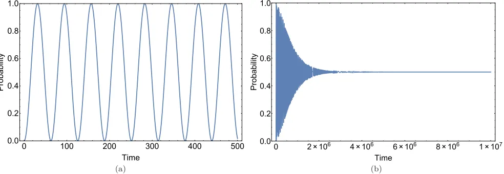
For an isolated macroscopic quantum system, the tunneling process, according to (4), is manifested by symmetrical oscillations between localized states of the system (FIG. 1-a). Since the system is isolated, such symmetrical oscillations are considered as the quantum signature of the system. A quantum system, especially a macroscopic one, is not actually isolated. An environment at thermal equilibrium destroys the quantum coherence between the preferred states of the system. This decoherence process is manifested in the reduction of the amplitude of oscillations, resulting to an equilibrium steady state at long times [37]. In our approach, if we eliminate one of the environments, the expected exponential decay of oscillations is observed (FIG. 1-b).
0 100 200 300 400 500
0.0 0.2 0.4 0.6 0.8 1.0
Time
Probability
(a)
0 2×10⁶ 4×10⁶ 6×10⁶ 8×10⁶ 1×10⁷
0.0 0.2 0.4 0.6 0.8 1.0
Time
Probability
(b)
FIG. 1: The dynamics of right-handed probability for the macroscopic quantum system withh = 10−1: a) for the isolated
system b) for the system in interaction with an equilibrium environment atT = 25K.
Now we turn to the case where the system interacts with two environments at the same temperatures. In order to compare the one-environment dynamics with the two-environment one, we divide the single equilibrium environment into two identical equilibrium environments. In doing so, we should note that, in two-environment dynamics, the effect of one environment is multiplied by the effect of the other one (see (26)). Hence, to retain the whole environment intact, the multiplication of coupling strengths and the addition of cut-off strengths of two environments should be conserved. At the short-time limit of the dynamics, the interference between two environments is manifested as successive interference patterns (FIG. 2-a). Here, the symmetry of the interference patterns can be considered as the signature of the similarity of two environments. At the long-time limit, as expected, the steady state is finally reached. This is in accordance with the work of Li and co-workers, in which a three-level microscopic system in interaction with two heat baths with the same temperature returns to the equilibrium case [25]. Nonetheless, if we compare the one-environment decoherence time (FIG. 1b) with the two-environment one (FIG. 2a), we realize that the interference between two environments through the system intensifis the decoherence process.
0 200 400 600 800 1000
0.0 0.2 0.4 0.6 0.8 1.0
Time
Probability
(a)
0 200 400 600 800 1000
0.0 0.2 0.4 0.6 0.8 1.0
Time
Probability
(b)
FIG. 2: The dynamics of right-handed probability for the macroscopic quantum system withh= 10−1 in interaction with two
The system being macroscopic exerts a force on environmental particles, which is realized by the second term of (6). It would be interesting to examine the effect of this back-action on the system’s dynamics. The comparison between the dynamics in the presence of this force (FIG. 2a) and in the absence of it (FIG. 2b) clearly shows that such a back-action weaken the interference between two environments.
The non-equilibrium environment is manifested here by considering two environments at different temperatures. Because of the non-trivial dynamics of the non-equilibrium environment, two consisting environments are not equivalent to a single equilibrium environment. At the short-time limit, the interference between two environments is observed in the dynamics (FIG. 3-a), but, unlike the same-temperature dynamics, the interference patterns are asymmetric. This asymmetry can be considered as the dynamical signature of the non-equilibrium environment. At the long-time limit, however, the non-equilibrium feature is suppressed and the system returns to its steady state. Also, the system’s back-action here wash off the interference between two environments (FIG. 3-b).
0 100 200 300 400
0.0 0.2 0.4 0.6 0.8 1.0
Time
Probability
(a)
0 100 200 300 400
0.0 0.2 0.4 0.6 0.8 1.0
Time
Probability
(b)
FIG. 3: The dynamics of right-handed probability for the macroscopic quantum system withh= 10−1 in interaction with a
non-equilibrium environment, consisting two environments atT
A= 1KandTB= 100Ka) with system’s back-action b) without system’s back-action.
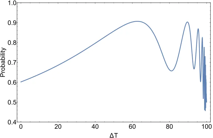
At a fixed temperature for the first environment, the right-handed probability in terms of the temperature difference between two environments ∆T =T1−T2 is plotted in FIG. 4. It shows that essentially the coherence of the system has an oscillatory dependence with ∆T. At first, for a wide range of temperatures, the coherence increases with ∆T. This is in agreement with the the work of Li and co-workers, in which the coherence increases with the temperature difference of two heat baths coupled to a three-state system [10]. According to our analysis, however, when this difference reaches to a critical value, the coherence is non-monotonically decreased. This is because after the critical point the decoherence feature of the hot environment dominates the process and the coherence is destroyed.
0 20 40 60 80 100
0.4 0.5 0.6 0.7 0.8 0.9 1.0
ΔT
Probability
FIG. 4: The right-handed probability in terms of the temperature difference between two environments ∆T = T
A−TB at
6. CONCLUSION
We examined the dynamics of a macroscopic quantum system in interaction with a non-equilibrium environment. Such an environment is minimally described by two independent equilibrium environments at different temperatures. It is believed that the dynamics of the system in interaction with two independent environments at same temperatures is reduced to that of a single equilibrium environment. However, we demonstrated that the interaction between two environments through the system manifests itself as successive interference patterns in the dynamics. In the non-equilibrium environment, it is claimed that the quantum coherence increases with the temperature difference between two environments. However, our analysis shows that this is not true for the large temperature differences. In fact, when the difference reaches a critical value, the decoherence feature of the hot environment dominates the process and thus the coherence is destroyed. We also examined how the macroscopic feature of the system is realized in the dynamics. In general, a quantum system exerts a force on environmental particles. This system’s back-action intensifies the decoherence process. The environment is usually considered to be large, so for a microscopic quantum system this force is negligible. For a macroscopic quantum system, however, this force affects the dynamics considerably. In fact, in the non-equilibrium environment, the coherence enhancement is decreased with the macroscopicity of the system.
ACKNOWLEDGEMENT
F.T.G acknowledges the financial support of Iranian National Science Foundation (INSF) for this work.
∗ Corresponding Author: [email protected]
[1] E. Jooset al. Decoherence and the Appearance of a Classical World in Quantum Theory, Springer-Verlag, Berlin, 2003. [2] M. A. Schlosshauer,Decoherence and the quantum-to-classical transition, Springer, Berlin, 2007.
[3] M. O. Scully, S.-Y. Zhu and A. Gavrielides,Phys. Rev. Lett.62, 2813, 1989. [4] M. O. Scully, M.S. Zubairy, G. S. Agarwal and H. Walther,Science299, 862, 2003. [5] H. T. Quan, P. Zhang and C.P. Sun,Phys. Rev. E73, 036122, 2006.
[6] S. De Liberato and M. Ueda,Phys. Rev. E84, 051122, 2011.
[7] H.-P. Breuer and F. Petruccione,The theory of open quantum systems, Oxford University Press, Oxford, 2002. [8] U. Weiss,Quantum Dissipative Systems, World Scientific, Singapore, 1999.
[9] J. Jing, Z. G. Lau and Z. Ficek,Phys. Rev. A79, 044305, 2009.
[10] Z. H. Li, D. W. Wang, H. Zheng, S. Y. Zhu and M. S. Zubairy,Phys. Rev. A80, 023801, 2009. [11] F. Caruso, A. W. Chin, A. Datta, S. F. Huelga and M. B. Plenio,J. Chem. Phys.131, 105106, 2009. [12] S. Yang, D. Z. Xu, Z. Song and C. P. Sun,J. Chem. Phys.132, 234501, 2010.
[13] J. Q. Liao, J. F. Huang, L. M. Kuang, C. P. Sun,Phys. Rev. A82, 052109, 2010. [14] Q. Ai, Y. Li, H. Zheng, and C. P. Sun,Phys. Rev. A 81, 042116, 2010.
[15] C. J. Myattet al. Nature403, 269, 2000.
[16] J. Schriefl, M. Clusel, D. Carpentier and P. Degiovanni,Europhys. Lett. 69, 156, 2005. [17] J. Schriefl, M. Clusel, D. Carpentier and P. Degiovanni,Phys. Rev. B 72, 035328, 2005. [18] H. Kohler, F. Sols,New J. Phys.8, 149, 2006.
[19] G. Gordon, G. Kurizki, S. Mancini, D. Vitali and P. Tombesi,J. Phys. B: Atom. Mol. Opt. Phys./bf 40, S61, 2007. [20] J. Clausen, G. Bensky and G. Kurizki,Phys. Rev. Lett.104, 040401, 2008.
[21] A. Montina and F. T. Arecchi,Phys. Rev. Lett100, 120401, 2008. [22] C. Emary,Phys. Rev. A78, 032105, 2008.
[23] J. Beer and E. Lutz, Decoherence in a Nonequilibrium Environment, arXiv:1004.3921, 2010. [24] C. C. Martens,J. Chem. Phys.133, 241101, 2010.
[25] S. W. Li, C.Y. Cai, C.P. Sun,Ann. Phys.360, 19, 2015.
[26] H. J. Moreno, T. Gorin and T. H. Seligman,Phys. Rev. A92, 030104(R), 2015. [27] M. Ludwig, K. Hammerer and F. Marquardt,Phys. Rev. A82, 012333, 2010. [28] J. C. Castillo, Ferney J. Rodriguez, L. Quiroga,Phys. Rev. A,88, 022104, 2013. [29] A. J. Leggett,J. Phys. Condens. Matter14, R415, 2002.
[30] M. Arndt and K. Hornberger,Nature Physics10, 271, 2014.
[31] P. Sekatski, N. Gisin and N. Sangouard,Phys. Rev. Lett.113, 090403, 2014. [32] A. J. Leggettet al. Rev. Mod. Phys.59, 1, 1987.
[33] S. Takagi, Macroscopic Quantum Tunneling, Cambridge University Press, Cambridge, 2002. [34] R. A. Harris and L. Stodolsky,J. Chem. Phys.74, 2145, 1981.
[35] R. A. Harris and L. Stodolsky,Phys. Lett. B,116, 164, 1982. [36] J. F. Dobson,Chem. Phys. Lett.61, 157, 1979.