Calculation of Rozansky-Witten Invariants
on the Hilbert Schemes of Points on a K3 Surface
and the Generalised Kummer Varieties
Marc A. Nieper-Wißkirchen1Received: September 1, 2003 Revised: December 19, 2003
Communicated by Thomas Peternell
Abstract. For any holomorphic symplectic manifold (X, σ), a closed Jacobi diagram with 2k trivalent vertices gives rise to a Rozansky-Witten class
RWX,σ(Γ)∈H2k(X,OX).
If X is irreducible, this defines a number βΓ(X, σ) by RWX,σ(Γ) =
βΓ(X, σ)[¯σ]k.
Let (X[n], σ[n]) be the Hilbert scheme of n points on a K3 surface together with a symplectic formσ[n] such thatR
X[n](σ[n]σ¯[n])n =n!.
Further, let (A[[n]], σ[[n]]) be the generalised Kummer variety of di-mension 2n −2 together with a symplectic form σ[[n]] such that
R
A[[n]](σ[[n]]σ¯[[n]])n =n!. J. Sawon conjectured in his doctoral thesis
that for every connected Jacobi diagram, the functionsβΓ(X[n], σ[n]) andβΓ(A[[n]], σ[[n]]) are linear inn.
We prove that this conjecture is true for Γ being a connected Jacobi diagram homologous to a polynomial of closed polywheels. We further show how this enables one to calculate all Rozansky-Witten invariants ofX[n] and A[[n]] for closed Jacobi diagrams that are homologous to a polynomial of closed polywheels. It seems to be unknown whether every Jacobi diagram is homologous to a polynomial of closed poly-wheels. If indeed the closed polywheels generate the whole graph homology space as an algebrea, our methods will thus enable us to computeall Rozansky-Witten invariants for the Hilbert schemes and the generalised Kummer varieties using these methods.
Also discussed in this article are the definitions of the various graph homology spaces, certain operators acting on these spaces and their relations, some general facts about holomorphic symplectic manifolds and facts about the special geometry of the Hilbert schemes of points on surfaces.
1The author is supported by the Deutsche Forschungsgemeinschaft. This work has been
2000 Mathematics Subject Classification: 53C26, 14Q15, 57M15, 05C99
Contents
1. Introduction 592
2. Preliminaries 594
2.1. Some multilinear algebra 594
2.2. Partitions 595
2.3. A lemma from umbral calculus 596
3. Graph homology 597
3.1. The graph homology space 597
3.2. Operations with graphs 600
3.3. Ansl2-action on the space of graph homology 603 3.4. Closed and connected graphs, the closure of a graph 604
3.5. Polywheels 606
4. Holomorphic symplectic manifolds 606
4.1. Definition and general properties 606
4.2. A pairing on the cohomology of a holomorphic symplectic
manifold 607
4.3. Example series 608
4.4. Aboutα[n] andα[[n]] 609
4.5. Complex genera of Hilbert schemes of points on surfaces 611
5. Rozansky-Witten classes and invariants 614
5.1. Definition 614
5.2. Examples and properties of Rozansky-Witten classes 615 5.3. Rozansky-Witten classes of closed graphs 616
6. Calculation for the example series 617
6.1. Proof of the main theorem 617
6.2. Some explicit calculations 620
References 622
1. Introduction
Every hyperk¨ahler manifold (X, g) can be given the structure of a K¨ahler manifold X (which is, however, not uniquely defined) whose K¨ahler metric is just given by g. X happens to carry a holomorphic symplectic two-form
σ ∈ H0(X,Ω2
X), whereas we shall call X a holomorphic symplectic manifold. Now M. Kapranov showed in [8] that one can in fact calculate bΓ(X) from (X, σ) by purely holomorphic methods.
The basic idea is the following: We can identify the holomorphic tangent bundle
TX ofX with its cotangent bundle ΩX by means ofσ. Doing this, the Atiyah class αX (see [8]) of X lies in H1(X,S3TX). Now we place a copy of αX at each trivalent vertex of the graph, take the ∪-product of all these copies (which gives us an element in H2k(X,(S3T
X)⊗2k) if 2kis the number of trivalent vertices), and finally contract (S3TX)⊗2k) along the edges of the graph by means of the holomorphic symplectic formσ. Let us call the resulting element RWX,σ(Γ)∈H2k(X,O
X). In case 2k is the complex dimension of X, we can integrate this element overX after we have multiplied it with [σ]2k. This gives us more or less bΓ(X). The orientation at the vertices of the graph is needed in the process to get a number which is not only defined up to sign.
There are two main example series of holomorphic symplectic manifolds, the Hilbert schemes X[n] of points on a K3 surface X and the generalised Kum-mer varieties A[[n]] (see [2]). Besides two further manifolds constructed by K. O’Grady in [13] and [12], these are the only known examples ofirreducible
holomorphic symplectic manifolds up to deformation.
Not much work was done on actual calculations of these invariants on the example series. The first extensive calculations were carried out by J. Sawon in his doctoral thesis [16]. All Chern numbers are in fact Rozansky-Witten invariants associated to certain Jacobi diagrams, calledclosed polywheels. Let
W be the subspace spanned by these polywheels in B. All Rozansky-Witten invariants associated to graphs lying in W can thus be calculated from the knowledge of the Chern numbers (which are computable in the case of X[n] ([3]) orA[[n]]([11]). However, from complex dimension four on, there are graph homology classes that do not lie inW. J. Sawon showed that for some of these graphs the Rozansky-Witten invariants can still be calculated from knowledge of the Chern numbers, which enables one to calculate all Rozansky-Witten invariants up to dimension five. His calculations would work for all irreducible holomorphic manifolds whose Chern numbers are known.
In this article, we will make use of the special geometry ofX[n]andA[[n]]. Doing this, we are able to give a method which enables us to calculate all Rozansky-Witten invariants for graphs homology classes that lie in thealgebraCgenerated byclosed polywheels in B. The closed polywheels form the subspaceW of the algebraBof graph homology. This is really a proper subspace. However,C, the algebra generated by this subspace, is much larger, and, as far as the author knows, it is unknown whether C = B, i.e. whether this work enables us to calculateall Rozanky-Witten invariants for the main example series.
The idea to carry out this computations is the following: Let (Y, τ) be any irreducible holomorphic symplectic manifold. Then H2k(Y,O
[¯τ]k. Therefore, every graph Γ with 2k trivalent vertices defines a number
βΓ(Y, τ) by RWY,τ(Γ) = βΓ(Y, τ)[¯τ]k. J. Sawon has already discussed how knowledge of these numbers for connected graphs is enough to deduce the values of all Rozansky-Witten invariants.
For the example series, let us fix holomorphic symplectic formsσ[n], respective
σ[[n]] with R
X[n](σ[n]σ¯[n])n =n! respective
R
A[[n]](σ[[n]]¯σ[[n]])n =n!. J. Sawon
conjectured the following:
The functions βΓ(X[n], σ[n]) and βΓ(X[[n]], σ[[n]]) are linear in
nfor Γ being a connected graph.
The main result of this work is the proof of this conjecture for the class of connected graphs lying in C (see Theorem 3). We further show how one can calculate these linear functions from the knowledge of the Chern numbers and thus how to calculate all Rozansky-Witten invariants for graphs inC.
We should note that we don’t make any use of the IHX relation in our deriva-tions, and so we could equally have worked on the level of Jacobi diagrams. Let us finally give a short description of each section. In section 2 we collect some definitions and results which will be used later on. The next section is concerned with defining the algebra of graph homology and certain operations on this space. We defineconnected polywheels and show how they are related with the usual closed polywheels in graph homology. We further exhibit a natural sl2-action on an extended graph homology space. In section 4, we first look at general holomorphic symplectic manifolds. Then we study the two example series more deeply. Section 5 defines Rozansky-Witten invariants while the last section is dedicated to the proof of our main theorem and explicit calculations.
2. Preliminaries
2.1. Some multilinear algebra. LetT be a tensor category (commutative and with unit). For any object V in T, we denote by SkV the coinvariants of
V⊗k with respect to the natural action of the symmetric group and by ΛkV the coinvariants with respect to the alternating action. Further, let us denote by SkV and ΛkV the invariants of both actions.
Proposition1. LetI be a cyclicly ordered set of three elements. LetV be an object in T. Then there exists a unique mapΛ3V →V⊗I such that for every
bijection φ : {1,2,3} → I respecting the canonical cyclic ordering of {1,2,3}
and the given cyclic ordering ofI the following diagram
Λ3V Λ3V
y
y V⊗3 −−−−→
φ∗
V⊗I (1)
Proof. Letφ, φ′:{1,2,3} →I be two bijections respecting the cyclic ordering. Then there exist an even permutationα∈A3such that the lower square of the following diagram commutes:
We have to show that the outer rectangle commutes. For this it suffices to show that the upper square commutes. In fact, sinceαis an even permutation, every element of Λ3V is by definition invariant underα∗. ¤
2.2. Partitions. A partitionλof a non-negative integern∈N0is a sequence
λ1, λ2, . . . of non-negative integers such that
Therefore almost allλi have to vanish. In the literature,λis often notated by 1λ12λ2. . .. The set of all partitions ofnis denoted by P(n). The union of all
Proof. We calculate
we have due to Proposition 2:
Proposition3. In Q[[s1, s2, . . .]][a1, a2, . . .]we have
2.3. A lemma from umbral calculus.
Lemma 1. Let R be any Q-algebra (commutative and with unit) and A(t)∈
So let us assume this special case for the rest of the proof. Let us denote byf(t) the compositional inverse ofB(t), i.e.f(B(t)) =t. We setg(t) :=A−1(f(t)). For the following we will make use of the terminology and the statements in [14]. Using this terminology, (10) states that (pn(x)) is the associated sequence to
Theorem 3.8.3 in [14] tells us that (sn(x−n)) is the Sheffer sequence to the pair (˜g(t),f˜(t)) with
˜
g(t) =g(t)(1 +f(t)/f′(t)) and
˜
f(t) =f(t) exp(t).
The compositional inverse of ˜f(t) is given by ˜B(t) :=B(WB(t)):
B(WB( ˜f(t))) =B(WB(f(t) exp(t))) =B(WB(f(t) exp(B(f(t))))) =B(f(t)) =t.
Further, we have ˜
A(t) := ˜g−1( ˜B(t))
= (g(B(t))(1 +f(B(t))/f′(B(t))))−1◦WB(t) = A(t)
1 +tB′(t)◦WB(t), which proves (13) again due to Theorem 2.3.4 in [14].
It remains to prove (12), i.e. that (xpn(x)
x−n ) is the associated sequence to ˜
f(t). We already know that (pn(x−n)) is the Sheffer sequence to the pair (1 +f(t)/f′(t),f˜(t)). By Theorem 2.3.6 of [14] it follows that the associated sequence to ˜f(t) is given by (1+f(d/dx)/f′(d/dx))p
n(x−n). By Theorem 2.3.7 and Corollary 3.6.6 in [14], we have
µ
1 + f(d/dx)
f′(d/dx)
pn(x−n) =pn(x−n) + 1
f′(d/dx)npn−1(x−n)
=pn(x−n) +npn(x−n)
x−n =
xpn(x−n)
x−n ,
which proves the rest of the lemma. ¤
3. Graph homology
This section is concerned with the space of graph homology classes of unitriva-lent graphs. A very detailed discussion of this space and other graph homology spaces can be found in [1]. Further aspects of graph homology can be found in [17], and, with respect to Rozansky-Witten invariant, in [7].
e
v3 v4
v1 v2
u1 u2
Figure 1. This Jacobi diagram has four trivalent vertices
v1, . . . , v4, and two univalent verticesu1 andu2, andeis one of its 7 edges.
Definition1. AJacobi diagram is a vertex-oriented graph with only uni- and trivalent vertices. A connected Jacobi diagram is a Jacobi diagram which is connected as a graph. Atrivalent Jacobi diagram is a Jacobi diagram with no univalent vertices.
We define thedegree of a Jacobi diagram to be the number of its vertices. It is always an even number.
We identify two graphs if they are isomorphic as vertex-oriented graphs in the obvious sense.
Example 1. The empty graph is a Jacobi diagram, denoted by 1. The unique Jacobi diagram consisting of two univalent vertices (which are connected by an edge) is denoted byℓ.
u1
u2
Figure 2. The Jacobi diagram ℓwith its two univalent ver-ticesu1andu2.
Remark 1. There are different names in the literature for what we call a “Ja-cobi diagram”, e.g. unitrivalent graphs, chord diagrams, Chinese characters, Feynman diagrams. The name chosen here is also used by D. Thurston in [17]. The name comes from the fact that the IHX relation in graph homology defined later is essentially the well-known Jacobi identity for Lie algebras.
With our definition of the degree of a Jacobi diagram, the algebra of graph homology defined later will be commutative in the graded sense. Further, the map RW that will associate to each Jacobi diagram a Rozansky-Witten class will respect this grading. But note that often the degree is defined to be half
of the number of vertices, which still is an integer.
of the flags at each trivalent vertex in the drawing to be the same as the given cyclic ordering.
Figure 3. These two graphs depict the same one.
In drawn Jacobi diagrams, we also use a notation like· · ·− · · ·n for a part of a graph which looks like a long line withnunivalent vertices (“legs”) attached to it, for example. . .⊥⊥⊥. . .forn= 3. The position ofnindicates the placement of the legs relative to the “long line”.
Definition 2. Let T be any tensor category (commutative and with unit). Every Jacobi diagram Γ with k trivalent and l univalent vertices induces a natural transformation ΨΓ between the functors
T → T,V 7→SkΛ3V ⊗SlV
(14)
and
T → T,V 7→SeS2V,
(15)
wheree:=3k+l
2 which is given by
(16) ΨΓ : SkΛ3V ⊗SlV (1)→O
t∈T
Λ3V ⊗O
f∈U
V (2)→O
t∈T
O
f∈t
V ⊗O
f∈U
V
(3)
→O
f∈F
V (4)→O
e∈E
O
f∈e
V (5)→SeS2V,
whereT is the set of the trivalent vertices,U the set of the univalent vertices,
F the set of flags, andE the set of edges of Γ. Further,
(1) is given by the natural inclusions of the invariants in the tensor prod-ucts,
(2) is given by the canonical maps (see Proposition 1 and recall that the setst are cyclicly ordered),
(3) is given by the associativity of the tensor product,
(4) is given again by the associativity of the tensor product, and finally (5) is given by the canonical projections onto the coinvariants.
Definition 3. We define B to be the Q-vector space spanned by all Jacobi diagrams modulo the IHX relation
=✁−✂
and the anti-symmetry (AS) relation
+✁= 0,
(18)
which can be applied anywhere within a diagram. (For this definition see also [1] and [17].) Two Jacobi diagrams are said to be homologous if they are in the same class modulo the IHX and AS relation.
Furthermore, let B′ be the subspace of Bspanned by all Jacobi diagrams not containing ℓ as a component, and let tB be the subspace of B′ spanned by all trivalent Jacobi diagrams. All these are graded and double-graded. The grading is induced by the degree of Jacobi diagrams, the double-grading by the number of univalent and trivalent vertices.
The completion of B (resp. B′, resp. tB) with respect to the grading will be denoted by ˆB (resp. ˆB′, resp.tBˆ).
We define Bk,l to be the subspace of ˆB generated by graphs with k trivalent andl univalent vertices. B′
k,l andtBk :=tBk,0 are defined similarly.
All these spaces are calledgraph homology spacesand their elements are called
graph homology classes orgraphs for short.
Remark 2. The subspaces Bk of ˆBspanned by the Jacobi diagrams of degree
k are always of finite dimension. The subspace B0 is one-dimensional and spanned by the graph homology class 1 of the empty diagram 1.
Remark 3. We have ˆB=Qk,l≥0Bk,l. In view of the following Definition 4, ˆB′ and ˆBare naturallyQ-algebras. AsQ-algebras, we have ˆB= ˆB′[[ℓ]]. Due to the AS relation, the spacesB′
k,lare zero forl > k. Therefore, ˆB′=
Q∞ k=0
Lk l=0B′k,l.
Example 2. Ifγis a graph which has a part looking like· · ·−· · ·n , it will become (−1)nγif we substitute the part· · ·− · · ·n by· · · −
n· · · due to the anti-symmetry relation.
3.2. Operations with graphs.
Definition 4. Disjoint union of Jacobi diagrams induces a bilinear map ˆ
B ×B →ˆ B,ˆ (γ, γ′)7→γ∪γ′.
(19)
By mapping 1∈Qto 1∈Bˆ, the space ˆBbecomes a gradedQ-algebra, which has no components in odd degrees. Often, we omit the product sign “∪”. B,
B′,tB, and so on are subalgebras.
Definition 5. Let k ∈ N. We call the graph homology class of the Jacobi diagram °2k the 2k-wheel w2k, i.e. w2 = ✂, w4 = ✄, and so on. It has 2k
univalent and 2ktrivalent vertices. The expressionw0will be given a meaning later, see section 3.3.
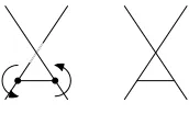
Let Γ be a Jacobi diagram and u, u′ be two different univalent vertices of Γ. These two should not be the two vertices of a component ℓof Γ. Let v (resp.
v′) be the vertexu(resp.u′) is attached to. The process ofgluing the vertices
u andu′ means to remove uand u′ together with the edges connecting them tovresp.v′and to add a new edge betweenvandv′. Thus, we arrive at a new graph Γ/(u, u′), whose number of trivalent vertices is the number of trivalent vertices of Γ and whose number of univalent vertices is the number of univalent vertices of Γ minus two. To make it a Jacobi diagram we define the cyclic orientation of the flags atv(resp.v′) to be the cyclic orientation of the flags at
v(resp.v′) in Γ with the flag belonging to the edge connectingv(resp.v′) with
u (resp. u′) replaced by the flag belonging to the added edge. For example,
u u′
Figure 4. Gluing the two univalent verticesu andu′ of the left graph produces the right one, denoted by 2.
gluing the two univalent vertices ofw2leads to the graph .
If π = {{u1, u′1}, . . . ,{uk, u′k}} is a set of two-element sets of legs that are pairwise disjoint and such that each pairuk, u′k fulfills the assumptions of the previous construction, we set
Γ/π:= Γ/(u1, u′1)/ . . . /(uk, u′k). (20)
Of course, the process of gluing two univalent vertices given above does not work ifuandu′ are the two univalent vertices ofℓ, thus our assumption on Γ. Definition6. Let Γ,Γ′ be two Jacobi diagrams, at least one of them without
ℓ as a component and U = {u1, . . . , un} resp. U′ the sets of their univalent vertices. We define
ˆ
Γ(Γ′) := X f:U ֒→U′ injective
(Γ∪Γ′)/(u1, f(u1))/ . . . /(un, f(un)), (21)
viewed as an element in ˆB.
This induces for everyγ∈BˆatBˆ-linear map ˆ
γ: ˆB′→Bˆ′, γ′ 7→ˆγ(γ′).
(22)
Example 3. Set ∂ := 12ℓˆ. It is is an endomorphism of ˆB′ of degree −2. For example,∂✂= . By setting
forγ, γ′∈Bˆ′, we have the following formula for allγ∈Bˆ′:
∂(γn) =
µ n
1
∂(γ)γn−1+
µ n
2
∂(γ, γ)γn−2.
(24)
This shows that ∂is a differential operator of order two acting on ˆB′.
Acting by ∂ on a Jacobi diagram means to glue two of its univalent vertices in all possible ways, acting by∂(·,·) on two Jacobi diagrams means to connect them by gluing a univalent vertex of the first with a univalent vertex of the second in all possible ways.
Definition7. Let Γ,Γ′ be two Jacobi diagrams, at least one of them without
ℓ as a component, and U ={u1, . . . , un} resp. U′ the sets of their univalent vertices. We define
hΓ,Γ′i:= X f:U→U′ bijective
(Γ∪Γ′)/(u1, f(u1))/ . . . /(un, f(un)), (25)
viewed as an element intBˆ. This induces atBˆ-bilinear map
h·,·i: ˆB′×B →ˆ tB,ˆ
(26)
which is symmetric on ˆB′×Bˆ′.
Note that hΓ,Γ′i is zero unless Γ and Γ′ have equal numbers of univalent vertices. In this case, the expression is the sum over all possibilities to glue the univalent vertices of Γ with univalent vertices of Γ′.
Note that hΓ,Γ′i is zero unless Γ and Γ′ have equal numbers of univalent vertices. In this case, the expression is the sum over all possibilities to glue the univalent vertices of Γ with univalent vertices of Γ′.
Proposition4. The maph1,·i: ˆB →tBˆis the canonical projection map, i.e.
it removes all non-trivalent components from a graph. Furthermore, forγ∈Bˆ′
andγ′∈Bˆ, we have
¿ γ,ℓ
2γ ′
À
=h∂γ, γ′i.
(27)
Forγ, γ′∈Bˆ′, we have the following (combinatorial) formula: (28) hexp(∂)(γγ′),1i=hexp(∂)γ,exp(∂)γ′i.
Proof. The formula (27) should be clear from the definitions.
Let us investigate (28) a bit more. We can assume that γ and γ′ are Jacobi diagrams with l resp.l′ univalent vertices andl+l′ = 2n withn∈N0. So we have to prove
∂n
n!(γγ ′) =
∞
X
m,m′=0 l−2m=l′−2m′
* ∂m
m!γ,
∂m′
m′!γ ′
sinceh·,1i: ˆB →tBˆmeans to remove the components with at least one univa-lent vertex. Recalling the meaning ofh·,·i, it should be clear that (28) follows from the fact that applying ∂k
k! on a Jacobi diagram means to glue all subsets of 2kof its univalent vertices tokpairs in all possible ways. ¤ 3.3. An sl2-action on the space of graph homology. In this short sec-tion we want to extend the space of graph homology slightly. This is mainly due to two reasons: When we defined the expression ˆΓ(Γ) for two Jacobi diagrams Γ and Γ′, we restricted ourselves to the case that Γ or Γ′ does not contain a component with anℓ. Secondly, we have not given thezero-wheelw0a meaning yet.
We do this by adding an element °to the various spaces of graph homology. Definition 8. The extended space of graph homology is the space ˆB[[°]]. Further, we set w0:=°, which, at least pictorially, is in accordance with the definition ofwk fork >0.
Note that this element is not depicting a Jacobi diagram as we have defined it. Nevertheless, we want to use the notion that ° has no univalent and no trivalent vertices, i.e. the homogeneous component of degree zero of ˆB[[°]] is Q[[°]].
When defining Γ/(u, u′) for a Jacobi diagram Γ with two univalent verticesu andu′, i.e. gluingutou′, we assumed thatuandu′ are not the vertices of one component ℓ of Γ. Now we extend this definition by defining Γ/(u, u′) to be the extended graph homology class we get by replacing ℓwith°, wheneveru
andu′ are the two univalent vertices of a componentℓof Γ.
Doing so, we can give the expression ˆγ(γ′)∈Bˆ[[°]] a meaning with no restric-tions on the two graph homology classesγ, γ′ ∈Bˆ, i.e. everyγ∈Bˆ[[°]] defines a tBˆ[[°]]-linear map
(29) γˆ: ˆB[[°]]→Bˆ[[°]].
Example 4. We have
(30) ∂ℓ=°.
Remark 5. We can similarly extend h·,·i: ˆB′×B →ˆ tBˆ to atBˆ[[°]]-bilinear form
(31) h·,·i: ˆB[[°]]×Bˆ[[°]]→tBˆ[[°]].
Bothℓ/2 and∂are two operators acting on the extended space of graph homol-ogy, the first one just multiplication withℓ/2. By calculating their commutator, we show that they induce a natural structure of ansl2-module on ˆB[[°]]. Proposition5. Let H : ˆB[[°]]→Bˆ[[°]]be the linear operator which acts on
γ∈Bˆk,l[[°]]by
(32) Hγ =
µ
1 2 °+l
We have the following commutator relations inEnd ˆB[[°]]:
[ℓ/2, ∂] =−H,
(33)
[H, ℓ/2] = 2·ℓ/2,
(34)
and
[H, ∂] =−2∂,
(35)
i.e. the triple (ℓ/2,−∂, H)defines a sl2-operation onBˆ[[°]].
Proof. Equations (34) and (35) follow from the fact that multiplying by °
commutes withℓ/2 and∂, and from the fact thatℓ/2 is an operator of degree 2 with respect to the grading given by the number of univalent vertices, whereas
∂ is an operator of degree−2 with respect to the same grading. It remains to look at (33). Forγ∈Bˆk,l[[°]], we calculate
[ℓ, ∂]γ=ℓ∂(γ)−∂(ℓγ) =ℓ∂(γ)−∂(ℓ)γ−ℓ∂(γ)−∂(ℓ, γ) =− °γ−2lγ=−2Hγ.
(36)
¤
Remark 6. Since ˆB[[°]] is infinite-dimensional, we have unfortunately difficul-ties to apply the standard theory ofsl2-representations to thissl2-module. For example, there are no eigenvectors for the operatorH.
3.4. Closed and connected graphs, the closure of a graph. As the number of connected components of a Jacobi diagram is preserved by the IHX-and AS-relations each graph homology space inherits a grading by the number of connected components. For any k ∈ N0 we define Bk to be the subspace of B spanned by all Jacobi diagrams with exactly k connected components. Similarly, we definetBk, ˆBk,tBˆk.
We haveB=L∞k=0Bk withB0=Q·1. Analogous results hold fortB, ˆB,tBˆ. Definition 9. A graph homology classγ is calledclosed ifγ∈tBˆ. The class
γ is calledconnected ifγ∈Bˆ1. Theconnected component ofγ is defined to be pr1(γ) where pr1: ˆB=Q∞
i=0Bˆi→Bˆ1 is the canonical projection. The closure
hγiof γis defined byhγi:=hγ,exp(ℓ/2)i. Theconnected closurehhγiiof γis defined to be the connected component of the closurehγiofγ.
For every finite set L, we define P2(L) to be the set of partitions of L into subsets of two elements. With this definition, we can express the closure of a Jacobi diagram Γ as
hΓi= X π∈P2(L)
Γ/π.
(37)
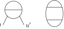
Example 5. We havehw2i= ,hhw2ii= ,
w2
2
®
= 2 2+ 2,
w2
2
®®
= 2 2. Let L1, . . . , Ln be finite and pairwise disjoint sets. We set L:=Fni=1Li. Let
π∈P2(L) be a partition ofLin 2-element-subsets. We say that a pairl, l′∈L
is linked by π if there is ani∈ {1, . . . n} such thatl, l′ ∈L
say thatπconnects the setsL1, . . . , Lnif and only if for each pairl, l′ ∈Lthere product over all these Jacobi diagrams. Let Li be the set of legs of Γi and denote byL:=Fni=1Li the set of all legs of Γ.
With this result we can prove the following Proposition:
Proposition6. For any connected graph homology classγ we have
exphhexpγii=hexpγi.
(40)
Note that both sides are well-defined in ˆB since γ and hh· · · ii as connected graphs have no component in degree zero.
Proof. Let Γ be any connected Jacobi diagram. By (39) we have
hΓni= X
3.5. Polywheels. by all polywheels is denoted by W and called the polywheel subspace. The subalgebra in tB spanned by all polywheels is denoted by C and called the
algebra of polywheels.
The connected closure hhw˜2λiiof ˜w2λ is called aconnected polywheel.
Remark 7. As discussed by J. Sawon in his thesis [16], W is proper graded subspace oftB. From degree eight on,tB
k is considerably larger thanWk. On the other hand it is unknown (at least to the author) if the inclusionC ⊆tBis proper.
Remark 8. The subalgebraC′intBspanned by all connected polywheels equals
C. This is since we can use (40) to express every polywheel as a polynomial of connected polywheels and vice versa.
Example 6. Using Proposition 6 we calculated the following expansions of the connected polywheels in terms of wheels:
hhw˜2ii=hw˜2i 4.1. Definition and general properties.
Definition 11. Aholomorphic symplectic manifold (X, σ) is a compact com-plex manifoldXtogether with an everywhere non-degenerate holomorphic two-form σ∈H0(X,Ω2
The holomorphic symplectic manifold (X, σ) is calledirreducibleif it is simply-connected and H0(X,Ω2
X) is one-dimensional, i.e. spanned byσ.
It follows immediately that every holomorphic symplectic manifoldX has triv-ial canonical bundle whose sections are multiples ofσn, and, therefore, vanish-ing first Chern class. In fact, all odd Chern classes vanish:
Proposition7. LetX be a complex manifold andE a complex vector bundle on X. If E admits a symplectic two-form, i.e. there exists a section σ ∈
H0(X,Λ2E∗)such that the induced morphism E→E∗ is an isomorphism, all
odd Chern classes ofE vanish.
Remark 9. That the odd Chern classes ofE vanish up to two-torsion follows immediately from the factc2k+1(E) =−c2k+1(E∗) fork∈N0.
The following proof using the splitting principle has been suggested to me by Manfred Lehn.
Proof. We prove the proposition by induction over the rank ofE. For rkE= 0, the claim is obvious.
By the splitting principle (see e.g. [5]), we can assume thatEhas a subbundle
L of rank one. Let L⊥ be the σ-orthogonal subbundle to L of E. Since σis symplectic, L⊥ is of rank n−1 and L is a subbundle of L⊥. We have the following short exact sequences of bundles on X:
0 −−−−→ L −−−−→ E −−−−→ E/L −−−−→ 0
and
0 −−−−→ L⊥/L −−−−→ E/L −−−−→ E/L⊥ −−−−→ 0.
Sinceσinduces a symplectic form onL⊥/L, by induction, all odd Chern classes of this bundle of rank rkE−2 vanish. Furthermore, note that σ induces an isomorphism between Land (E/L⊥)∗, so all odd Chern classes of L⊕E/L⊥
vanish.
Now, the two exact sequences give usc(E) =c(L⊕E/L⊥)·c(L⊥/L). Therefore, we can conclude that all odd Chern classes ofE vanish. ¤
Proposition 8. For any irreducible holomorphic symplectic manifold(X, σ)
of dimension 2n and k ∈ 0, . . . , n the space H2k(X,OX) is one-dimensional
and spanned by the cohomology class [¯σ]k.
Proof. See [2]. ¤
4.2. A pairing on the cohomology of a holomorphic symplectic manifold. Let (X, σ) be a holomorphic symplectic manifold. There is a nat-ural pairing of coherent sheafs
As the natural morphism from Λ∗TX to Λ∗TX is an isomorphism and Λ∗TX can be identified with Λ∗ΩX by means of the symplectic form, we therefore have a natural map
Λ∗Ω⊗Λ∗ΩX → OX. (44)
We write
h·,·i: Hp(X,Ω∗)⊗Hq(X,Ω∗)→Hp+q(X,OX),(α, β)7→ hα, βi (45)
for the induced map for anyp, q∈N0. In [10] we proved the following proposition: Proposition9. For any α∈H∗(X,Ω∗) we have
Z
X
αexpσ=
Z
X
hα,expσiexpσ.
(46)
4.3. Example series. There are two main series of examples of irreducible holomorphic symplectic manifolds. Both of them are based on the Hilbert schemes of points on a surface:
Let X be any smooth projective surface over C and n ∈ N0. By X[n] we denote the Hilbert scheme of zero-dimensional subschemes of length n of X. By a result of Fogarty ([4]), X[n] is a smooth projective variety of dimension 2n. The Hilbert scheme can be viewed as a resolutionρ:X[n] →X(n)of the
n-fold symmetric product X(n) :=Xn/Sn. The morphismρ, sending closed points, i.e. subspaces of X, to their support counting multiplicities, is called the Hilbert-Chow morphism.
Letα∈H2(X,C) be any class. The classPn
i=1pr∗iα∈H2(Xn,C) is invariant under the action of Sn, where pri : Xn → X denotes the projection on the
ith factor. Therefore, there exists a class α(n) ∈ H2(X(n),C) with π∗α(n) =
Pn
i=1pr∗iα, where π : Xn → X(n) is the canonical projection. Usingρ this induces a classα[n] in H2(X[n],C).
IfXis a K3 surface or an abelian surface, there exists a holomorphic symplectic form σ∈ H2,0(X)⊆ H2(X,C). It was shown by Beauville in [2] thatσ[n] is again symplectic, so (X[n], σ[n]) is a holomorphic symplectic manifold.
Example 7. For any K3 surface X and holomorphic symplectic form σ ∈
H2,0(X), the pair (X[n], σ[n]) is in fact an irreducible holomorphic symplec-tic manifold.
This has also been proven by Beauville. In the case of an abelian surface A, we have to work a little bit more as A[n] is not irreducible in this case: LetAbe an abelian surface and let us denote bys:A[n] →Athe composition of the summation morphism A(n) → A with the Hilbert-Chow morphism ρ:
A[n]→A(n).
Definition 12. For anyn∈N, thenth generalised Kummer variety A[[n]] is the fibre ofsover 0∈A. For any classα∈H2(A,C), we setα[[n]]:=α[n]|
Example 8. For every abelian surface A and holomorphic symplectic form
σ ∈ H2,0(A), the pair (A[[n]], σ[[n]]) is an irreducible holomorphic symplectic manifold of dimension 2n−2.
The proof can also be found in [2].
4.4. About α[n] andα[[n]]. LetX be any smooth projective surface andn∈ N0.
LetX[n,n+1]denote the incidence variety of all pairs (ξ, ξ′)∈X[n]×X[n+1]with
ξ ⊆ξ′ (see [3]). We denote by ψ:X[n,n+1]→X[n+1]and by φ :X[n,n+1] →
X[n] the canonical maps. There is a third canonical map χ : X[n,n+1] → X mapping (ξ, ξ′)7→xifξ′ is obtained by extendingξat the closed pointx∈X. Proposition10. For any α∈H2(X,C)we have
ψ∗α[n+1]=φ∗α[n]+χ∗α.
(47)
Proof. Letp:X(n)×X →X(n) andq:X(n)×X →X denote the canonical projections. Letτ :X(n)×X →X(n+1) the obvious symmetrising map. The following diagram
X[n,n+1] X[n,n+1]
(φ,χ)
y
yψ X[n]×X X[n+1]
ρ×idX
y
yρ′ X(n)×X −−−−→τ X(n+1)
π×idX
x
x π′
Xn+1 Xn+1
is commutative. (Note that we have primed some maps to avoid name clashes.) We claim thatτ∗α(n+1)=p∗α(n)+q∗α. In fact, since
(π×idX)∗τ∗α(n+1)=π′∗α(n+1)= n+1
X
i=1 pr∗iα,
this follows from the definition of α(n). Finally, we can read off the diagram that
ψ∗α[n+1]=ψ∗ρ′∗α(n+1)= (φ, χ)∗(ρ×idX)∗τ∗α(n+1)
= (φ, χ)∗(ρ×idX)∗(p∗α(n)+q∗α) =φ∗α[n]+χ∗α.
Proposition 11. Let X = X1⊔X2 be the disjoint union of two projective
Proof. The splitting ofX[n] follows from the universal property of the Hilbert scheme and is a well-known fact. The statement on α[n] is easy to prove and so we shall only give a sketch: Let us denote by i:X[n1]
1 ×X [n2]
2 →X[n] the natural inclusion. Furthermore letj:X(n1)
1 ×X (n2)
2 →X(n)denote the natural symmetrising map. The following diagram is commutative:
X[n1]
i are the Hilbert-Chow morphisms. Sincej∗α(n)= pr∗
1α (n1)
1 + pr∗2α (n2)
2 , the commutativity of the diagram proves the statement
onα[n]. ¤
Let A be again an abelian surface and n ∈ N. Since A acts on itself by translation, there is also an induced operation of A on the Hilbert scheme
A[n]. Let us denote the restriction of this operation to the generalised Kummer varietyA[[n]]byν:A×A[[n]]→A[n]. It fits into the following cartesian square:
where s is the summation map as having been defined above and n : A → A, a7→nais the (multiplication-by-n)-morphism. Sincenis a Galois cover of degreen4, the same holds true forν.
Proposition12. For any α∈H2(A,C), we have
ν∗α[n]=npr∗1α+ pr∗2α[[n]]. (52)
Proof. By the K¨unneth decomposition theorem, we know thatν∗α[n] splits:
Setι1:A→A×A[[n]], a7→(a, ξ0) andι2:A[[n]]→A×A[[n]], ξ7→(0, ξ), where
ξ0is any subscheme of lengthnconcentrated in 0. We have
α1=ι∗1ν∗α[n]= (ρ◦ν◦ι1)∗α(n)= (a7→(a, . . . a
| {z }
n
))∗α(n)=nα
(53)
and
α2=ι∗2ν∗α[n] =i∗α[n]=α[[n]], (54)
where i:A[[n]]→A[n] is the natural inclusion map, thus proving the
proposi-tion. ¤
4.5. Complex genera of Hilbert schemes of points on surfaces. The following theorem is an adaption of Theorem 4.1 of [3] to our context.
Theorem 1. Let P be a polynomial in the variables c1, c2, . . . and α over Q. There exists a polynomial P˜ ∈Q[z1, z2, z3, z4] such that for every smooth
projective surfaceX,α∈H2(X,Q)andn∈N
0 we have:
Z
X[n]
P(c∗(X[n]), α[n]) = ˜P µZ
X
α2/2, Z
X
c1(X)α, Z
X
c1(X)2/2, Z
X
c2(X)
¶ .
(55)
Proof. The proof goes along the very same lines as the proof of Proposition 0.5 in [3] (see there). The only new thing we need is Proposition 10 of this paper to be used in the induction step of the adapted proof of Proposition 3.1 of [3]
to our situation. ¤
LetRbe anyQ-algebra (commutative and with unit) and letφ∈R[[c1, c2, . . .]] be a non-vanishing power series in the universal Chern classes such that φis multiplicative with respect to the Whitney sum of vector bundles, i.e.
φ(E⊕F) =φ(E)φ(F) (56)
for all complex manifolds and complex vector bundles E and F on X. Any
φ with this property induces a complex genus, also denoted byφ, by setting
φ(X) := RXφ(TX) for X a compact complex manifold. Let us call such a φ
multiplicative.
Remark 11. By Hirzebruch’s theory of multiplicative sequences and complex genera ([6]), we know that
(1) each complex genus is induced by a unique multiplicativeφ, and (2) the multiplicative elements in R[[c1, c2, . . .]] are exactly those of the
form exp(P∞k=1aksk) withak ∈R.
More or less formally the following theorem follows from Theorem 1.
Theorem 2. For each multiplicative φ ∈ R[[c1, c2, . . .]], there exist unique
have:
Proof. This theorem is again an adaption of a theorem (Theorem 4.2) of [3] to our context. Nevertheless, let us give the proof here:
Set K := ©(X, α) :X is a smooth projective surface andα∈H2(X,C)ª and letγ :K →Q4 be the map (X, α)7→(α2/2, c1(X)α, c1(X)2/2, c2(X)). Here, we have supressed the integral signs RX and interpret the expressionsα2, etc. as intersection numbers onX. The image ofKspans the wholeQ4(for explicit generators, we refer to [3]).
Now let us assume that a (X, α) ∈ K decomposes as (X, α) = (X1, α1)⊔ that loghis a linear function which proves the first part of the theorem. To get the first terms of the power series, we expand both sides of (57). The left hand side expands as
1 + (α2/2 +φ1c1(X)α+
while the right hand side expands as
where A1, B1, C1, D1 are the linear coefficients of Aφ, Bφ,Cφ, andDφ, which can therefore be read off by comparing the expansions. ¤
Corollary 1. Let X be any smooth projective surface, α ∈ H2(X,C), and
which proves the first part of the corollary by comparing coefficients ofq. For the Kummer case, we calculate
Z
which proves the rest of the corollary. ¤
Let ch be the universal Chern character. By sk = (2k)!ch2k we denote its components. They span the whole algebra of characteristic classes, i.e. we have Q[s1, s2, . . .] =Q[c1, c2, . . .].
Let us fix the power series
φ:= exp( ∞
X
k=1
a2ks2ktk)∈Q[a2, a4, . . .][t][[c1, c2, . . .]].
This multiplicative series gives rise to four power series
Aφ(p), Bφ(p), Cφ(p), Dφ(p)∈pR[[p]]
according to the previous Theorem 2. We shall set for the rest of this article
A(t) :=Aφ(1), and D(t) :=Dφ(1) (64)
The constant terms of these power series int are given by
A(t) = 1 +O(t), and D(t) =O(t).
5. Rozansky-Witten classes and invariants
The idea to associate to every graph Γ and every hyperk¨ahler manifold X a cohomology class RWX(Γ) is due to L. Rozansky and E. Witten (c.f. [15]). M. Kapranov showed in [8] that the metric structure of a hyperk¨ahler man-ifold is not nessessary to define these classes. It was his idea to build the whole theory upon the Atiyah class and the symplectic structure of an irre-ducible holomorphic symplectic manifold. We will make use of his definition of Rozansky-Witten classes in this section. A very detailed text on defining Rozansky-Witten invariants is the thesis by J. Sawon [16].
5.1. Definition. Let (X, σ) be a holomorphic symplectic manifold. Let us work in the category of complexes of coherent sheaves onX. In this category, we have for everyn∈Za functorV 7→V[n] that shifts a complexV bynto the left. Due to the Koszul sign rule (i.e. the natural map (V[m])⊗(W[n])→
(W[n])⊗(V[m]) for sheaves V and W and integers n and m incorporates a sign (−1)mn), we have Sn(V[1]) = (ΛnV)[n] and Sn(V[1]) = (ΛnV)[n].
Every Jacobi diagram Γ withktrivalent andl univalent vertices defines in the category of complexes of coherent sheaves onX a morphism
ΦΓ: SkΛ3(TX[−1])⊗Sl(TX[−1])→SeS2(TX[−1]), (66)
whereTX[−1] is the tangent sheaf ofX shifted by one and 2e= 3k+l. By the sign rule above, this is equivalent to being given a map:
(ΛkS3TX⊗ΛlTX)[−3k−l]→(SeΛ2TX)[−2e], (67)
which is induced by a map
ΛkS3TX⊗ΛlTX →SeΛ2TX (68)
in the category of coherent sheaves on X. This gives rise to a map ΨΓ : ΛkS3TX⊗SeΛ2ΩX →ΛlΩX.
(69)
Let ˜α ∈ H1(X,Ω⊗EndTX) be the Atiyah class of X, i.e. ˜α represents the extension class of the sequence
0 −−−−→ ΩX⊗ TX −−−−→ J1TX −−−−→ TX −−−−→ 0 (70)
in Ext1X(TX,ΩX⊗ TX) = H1(X,ΩX ⊗EndTX). Here, J1TX is the bundle of one-jets of sections ofTX (for more on this, see [8]). The Atiyah class can also be viewed as the obstruction for a global holomorphic connection to exist on
TX. We setα:=i/(2π)˜α.
We use σ to identify the tangent bundle TX of X with its cotangent bundle ΩX. Doing this,αcan be viewed as an element of H1(X,T⊗3
X ). Now the point is that α is not any such element. The following proposition was proven by Kapranov in [8]:
Proposition13.
Therefore, α∪k∪σ∪l∈ Hk(X,ΛkS3T
X⊗SlΛ2ΩX). Applying the map ΨΓ on the level of cohomology eventually leads to an element
RWX,σ(Γ) := ΨΓ∗(α∪k∪σ∪l)∈Hk(X,ΩlX). (72)
We call RWX,σ(Γ) theRozansky-Witten class of (X, σ)associated to Γ. For aC-linear combinationγof Jacobi diagrams, RWX,σ(γ) is defined by linear extension.
In [8], Kapranov also showed the following proposition, which is crucial for the next definition. It follows from a Bianchi-identity for the Atiyah class.
Proposition 14. If γ is a Q-linear combination of Jacobi diagrams that is zero modulo the anti-symmetry and IHX relations, then RWX,σ(γ) = 0.
Definition 13. We define a double-graded linear map RWX,σ : ˆB →H∗(X,Ω∗X), (73)
which maps Bk,l into Hk(X,ΩlX) by mapping a homology class of a Jacobi diagram Γ to RWX,σ(Γ).
Definition 14. Letγ∈Bˆbe any graph. The integral
bγ(X, σ) :=
Z
X
RWX,σ(γ) exp(σ+ ¯σ) (74)
is called theRozansky-Witten invariant of(X, σ) associated toγ.
5.2. Examples and properties of Rozansky-Witten classes. We sum-marise in this subsection the properties of the Rozansky-Witten classes that will be of use for us. For proofs take a look at [10], please.
Let (X, σ) again be a holomorphic symplectic manifold.
Proposition 15. The map RWX,σ : ˆB → H∗,∗(X) is a morphism of graded
algebras.
Proposition16. For all γ∈Bˆ′ andγ′∈Bˆwe have RWX,σ(hγ, γ′i) =hRWX,σ(γ),RWX,σ(γ′)i. (75)
Example 9. The cohomology class [σ] ∈H2,0(X) is a Rozansky-Witten class; more precisely, we have
RWX,σ(ℓ) = 2[σ].
(76)
Example 10. The components of the Chern charakter are Rozansky-Witten invariants:
−RWX,σ(w2k) = RWX,σ( ˜w2k) =s2k. (77)
The next two proposition actually aren’t stated in [10], so we shall give ideas of their proofs here.
Proposition 17. Let ν : (X, ν∗σ)→(Y, σ)be a Galois cover of holomorphic
symplectic manifolds. For every graph homology classγ∈Bˆ,
Proof. As ν is a Galois cover, we can identify TX withν∗TY and so ˜αX with
ν∗α˜
Y where ˜αX and ˜αY are the Atiyah classes of X and Y. By definition of
the Rozansky-Witten classes, (78) follows. ¤
Lemma 2. Let (X, σ) and(Y, τ) be two holomorphic symplectic manifolds. If the tangent bundle of Y is trivial,
RWX×Y,p∗σ+q∗τ(γ) =p∗RWX,σ(γ) (79)
for all graphs γ ∈ Bˆ′. Here p:X ×Y →X andq : X×Y →Y denote the
canonical projections.
Proof. This lemma is a special case of the more general proposition in [16] that relates the coproduct in graph homology with the product of holomorphic symplectic manifolds. Since all Rozansky-Witten classes for graphs with at least one trivalent vertex vanish onY, our lemma follows easily from J. Sawon’s
statement. ¤
5.3. Rozansky-Witten classes of closed graphs. Letγ be a homoge-neous closed graph of degree 2k. For every compact holomorphic symplectic manifold (X, σ), we have RWX,σ(γ)∈H0,2k(X). IfX is irreducible, we there-fore have RWX,σ(γ) = βγ ·[¯σ]k for a certain βγ ∈ C. We can express βγ as
βγ=
R
XRWX,σ(γ)¯σ n−kσn
R
X(σσ¯)n
=(n−k)!
n!
R
XRWX,σ(γ) exp(σ+ ¯σ)
R
Xexp(σ+ ¯σ) (80)
where 2nis the dimension ofX.
This formula makes also sense for non-irreducible X, which leads us to the following definition:
Definition 15. Let (X, σ) be a compact holomorphic symplectic manifold (X, σ) of dimension 2n. For any homogeneous closed graph homology classγ
of degree 2kwith k≤nwe set
βγ(X, σ) :=
(n−k)!
n!
R
XRWX,σ(γ) exp(σ+ ¯σ)
R
Xexp(σ+ ¯σ) (81)
By linear extension, we can define βγ(X, σ) also for non-homogeneous closed graph homology classesγ.
Remark 12. The maptB →ˆ C, γ 7→β
γ(X, σ) is linear. IfX is irreducible, it is also a homomorphism of rings.
For polywheels ˜w2λ, we can expressβhw˜2λiin terms of characteristic classes:
Proposition18. Let(X, σ)be a compact holomorphic symplectic manifold of dimension 2n andk∈ {1, . . . , n}. Letλ∈P(k)be any partition of k. Then
Z
X
RWX,σ(hw˜2λi) exp(σ+ ¯σ) =
Z
X
s2λ(X) exp(σ+ ¯σ).
Proof. We calculate
(83)
Z
X
RWX,σ(hw˜2λi) exp(σ+ ¯σ) =
Z
X
RWX,σ(hw˜2λ,exp(ℓ/2)i) exp(σ+ ¯σ)
=
Z
X
hs2λ,expσiexp(σ+ ¯σ) =
Z
X
s2λexp(σ+ ¯σ).
¤
6. Calculation for the example series
6.1. Proof of the main theorem. Let X be a smooth projective surface that admits a holomorphic symplectic form (e.g. a K3 surface or an abelian surface). Let us fix a holomorphic symplectic form σ ∈H2,0(X) that is nor-malised such that RXσσ¯ = 1. It is known ([9]) that X[n] for alln ∈ N0 is a compact holomorphic symplectic manifold.
For every homogeneous closed graph homology classγ of degree 2k and every
n∈N0, we set
hXγ (n) :=βγ(X[k+n], σ[k+n]). (84)
By linear extension, we define hX
γ (n) for non-homogeneous closed graph ho-mology classes γ.
Proposition19. For all closed graph homology classes γ, we have
∞
X
n=0
qn
n!h X γ (n) =
∞
X
l=0
Z
X[l]
RWX[l],σ[l](γ) exp(q 1
2(σ[l]+ ¯σ[l]))
(85)
in C[[q]].
Proof. Let us assume thatγ is homogeneous of degree 2k. Then
hX
γ(n) =βγ(X[k+n], σ[k+n]) =
n! (n+k)!
R
X[k+n]RWX[k+n],σ[k+n](γ) exp(σ[k+n]+ ¯σ[k+n])
R
X[k+n]exp(σ[k+n]+ ¯σ[k+n])
=n!
Z
X[k+n]
RWX[k+n],σ[k+n](γ) exp(σ+ ¯σ).
In the last equation we have used Corollary 1. Summing up and introducing
the counting parameterq yields the claim. ¤
Proposition20. Let a2, a4, . . . be formal parameters. We set
ω(t) := ∞
X
k=1
and call ω the universal wheel. Further, we setW(t) := exp(ω(t))and W :=
W(1). The Rozansky-Witten classes of the universal wheel are encoded by
∞
Proof. Using Proposition 19 and Proposition 18 yields: ∞
Corollary 2. For everyn∈N0 we have
hXhW(t)i(n) = exp(c2(X)D(t)) exp(nlogA(t)) (88)
Proof. Comparision of coefficients in (87) gives
hXhW(t)i(n) =A(t)nexp(c2(X)D(t)).
Lastly, note thatAis a power series int that has constant coefficient one. ¤
Remark 13. By equation (88) we shall extend the definition of hX
hW(t)i(n) to alln∈Z.
Proposition 21. Let Abe an abelian surface. Let us fix a holomorphic sym-plectic form σ∈H2,0(A)that is normalised such thatRAσσ¯= 1.
Let γ be a homogeneous connected closed graph of degree2k. Then we have
βγ(A[[n]], σ[[n]]) =
Proof. The proof is a straight-forward calculation:
βγ(A[[n]], σ[[n]]) = (n−1−k)!
Theorem3. For any homogenous connected closed graph of degree2klying in the algebraC of polywheels there exist two rational numbersaγ, cγ such that for
each K3 surfaceX together with a symplectic formσ∈H2,0(X)withR
Xσσ¯= 1
andn≥k we have
βγ(X[n], σ[n]) =aγn+cγ (90)
and that for each abelian surfaceAtogether with a symplectic formσ∈H2,0(X)
with RXσ¯σ= 1and n > kwe have
βγ(A[[n]], σ[[n]]) =aγn. (91)
Proof. Let (X, σ) be a K3 surface or an abelian surface together with a sym-plectic form with RXσσ¯ = 1. Let W2k be the homogeneous component of sition 6 and Remark 12 we therefore have
βhhW(t)ii(X[n], σ[n]) =βloghW(t)i(X[n], σ[n]) = logβhW(t)i=nV˜(t) + logU(t). Finally, let λbe any partition. Setting
∂2λ:=
Let us now turn to the case of a generalised Kummer variety, i.e. let X =A
be an abelian surface and n≥1. Note thatc2(A) = 0. Here, we have due to Proposition 21:
βhW2ki(A
[[n]], σ[[n]]) = n
n−kh
A
hW2ki(n−k)
forn > k. Forn≤kwe take this equation as a definition for its left hand side. AsU0(t) = 1, Lemma 1 yields in this case that
βhW(t)i(A[[n]], σ[[n]]) = ∞
X
k=0
n n−kh
X
hW2ki(n−k)t
k = expnV˜(t).
We can then proceed as in the case of the Hilbert scheme of a K3 surface to finally get
βhhw˜2λii=n∂2λ( ˜V(t)).
¤
6.2. Some explicit calculations. Now, we’d like to calculate the constants
aγ and cγ for any homogeneous connected closed graph homology class γ of degree 2klying in C. By the previous theorem, we can do this by calculating
βγ on (X, σ) for (X, σ) being the 2k-dimensional Hilbert scheme of points on a K3 surface and the 2k-dimensional generalised Kummer variety.
We can do this by recursion over k: Let the calculation having been done for homogeneous connected closed graph homology classesγof degree less than 2k
in Cand both example series.
Letλbe any partition ofk. We can expresshhw˜2λiias
hhw˜2λii=hw˜2λi+P, (94)
where P is a polynomial in homogeneous connected closed graph homology classes γ of degree less than 2k in C (for this see Proposition 6). Therefore,
βhhw˜2λii(X, σ) is given by
βhhw˜2λii(X, σ) =βhw˜2λi(X, σ) +P
′, (95)
where P′ is a polynomial in terms like β
γ′(X, σ) with γ′ ∈ C and degγ′ < 2k. However, these terms have been calculated in previous recursion steps. Therefore, the only thing new we have to calculate in this recursion step is
βhw˜2λi(X, σ). We have:
βhw˜2λi(X, σ) =
1
k!
R
XRWX,σ( ˜w2λ) exp(σ+ ¯σ)
R
Xexp(σ+ ¯σ)
=
R
Xs2λ(X)
R
Xexp (σ+ ¯σ)
.
(96)
As all the Chern numbers ofXcan be computed with the help of Bott’s residue formula (see [3] for the case of the Hilbert scheme and [11] for the case of the generalised Kummer variety), we therefore are able to calculate βhw˜2λi(X, σ).
This ends the recursion step as we have given an algorithm to computeaγ and
We worked through the recursion fork= 1,2,3. Firstly, we have
Not let X be a K3 surface and A an abelian surface. Let us denote by σ
either a holomorphic symplectic two-form on X withRXσσ¯ = 1 or onAwith
R
Aσ¯σ= 1. We use the following table of Chern numbers for the Hilbert scheme of points on a K3 surface:
k s s[X[k]] s[A[[k+1]]]
Going through the recursion, we arrive at the following table:
k γ βγ(A[[k+1]]) βγ(X[k]) aγ cγ
Now, we would like to turn to Rozansky-Witten invariants: Let γ be any homogeneous closed graph homology class of degree 2k. For any holomorphic symplectic manifold (X, σ) of dimension 2n, the associated Rozansky-Witten invariant is given by
schemes of points on a K3 surface and the generalised Kummer varieties — as long asγis spanned by the connected polywheels.
By the procedure outlined above, Theorem 3 therefore enables us to compute all Rozansky-Witten invariants of the two example series associated to closed graph homology classes lying inC.
References
[1] Dror Bar-Natan. On the Vassiliev knot invariants.Topology, 34(2):423–472, 1995.
[2] Arnaud Beauville. Vari´et´es K¨ahleriennes dont la premi`ere classe de Chern est nulle.J. Differential Geom., 18(4):755–782, 1983.
[3] Geir Ellingsrud, Lothar G¨ottsche, and Manfred Lehn. On the cobordism class of the Hilbert scheme of a surface. J. Algebraic Geom., 10(1):81–100, 2001.
[4] John Fogarty. Algebraic families on an algebraic surface.Amer. J. Math, 90:511–521, 1968.
[5] William Fulton.Intersection Theory, volume 2 of3.Springer-Verlag, Berlin, 1998.
[6] Friedrich Hirzebruch. Neue topologische Methoden in der Algebraischen Geometrie. Ergebnisse der Mathematik und ihrer Grenzgebiete. Springer-Verlag, Berlin, 1962.
[7] Nigel Hitchin and Justin Sawon. Curvature and characteristic numbers of hyper-K¨ahler manifolds.Duke Math. J., 106(3):599–615, 2001.
[8] Mikhail Kapranov. Rozansky-Witten invariants via Atiyah classes. Com-pos. Math., 115(1):71–113, 1999.
[9] Shigeru Mukai. Symplectic structure on the moduli space of sheaves on an abelian or K3 surface.Invent. Math., 77:101–116, 1984.
[10] Marc Nieper-Wißkirchen. Hirzebruch-Riemann-Roch formulae on irre-ducible symplectic K¨ahler manifolds. To appear in: Journal of Algebraic Geometry.
[11] Marc Nieper-Wißkirchen. On the Chern numbers of Generalised Kummer Varieties.Math. Res. Lett., 9(5–6):597–606, 2002.
[12] Kieran O’Grady. A new six-dimensional irreducible symplectic manifold.
arXiv:math.AG/0010187.
[13] Kieran O’Grady. Desingularized moduli spaces of sheaves on a K3.J. Reine Angew. Math., 512:49–117, 1999.
[14] Steven Roman. The Umbral Calculus. Pure and Applied Mathematics. Academic Press, Inc., Orlando, 1984.
[15] Lev Rozansky and Edward Witten. Hyper-K¨ahler geometry and invariants of three-manifolds.Selecta Math. (N.S.), 3(3):401–458, 1997.
[16] Justin Sawon. Rozansky-Witten invariants of hyperk¨ahler manifolds. PhD thesis, University of Cambridge, October 1999.
[18] Shing-Tung Yau. On the Ricci curvature of a compact K¨ahler manifold and the complex Monge-Amp`ere equations. I. Comm. Pure Appl. Math., 31:339–411, 1978.
Marc A. Nieper-Wißkirchen
Johannes Gutenberg-Universit¨at Mainz Fachbereich f¨ur Mathematik
und Informatik 55099 Mainz Germany