23 11
Article 00.2.4
Journal of Integer Sequences, Vol. 3 (2000),
23 6 1 47
On Generalizations of the Stirling Number Triangles
1
Wolfdieter Lang
Institut f¨
ur Theoretische Physik
Universit¨at Karlsruhe
Kaiserstraße 12, D-76128 Karlsruhe, Germany
Email address:
Home page:
http://www-itp.physik.uni-karlsruhe.de/˜ wl
Abstract
Sequences of generalized Stirling numbers of both kinds are introduced. These sequences of triangles (i.e. infinite-dimensional lower triangular matrices) of numbers will be denoted by S2(k;n, m) and S1(k;n, m) withk∈Z. The original Stirling number triangles of the second and first kind arise whenk= 1. S2(2;n, m) is identical with the unsignedS1(2;n, m)triangle, called S1p(2;n, m), which also represents the triangle of signless Lah numbers. Certain associated number triangles, denoted by s2(k;n, m)ands1(k;n, m), are also defined. Both s2(2;n, m) and s1(2;n+ 1, m+ 1) form Pascal’s triangle, and s2(−1, n, m)turns out to be Catalan’s triangle.
Generating functions are given for the columns of these triangles. Each S2(k)and S1(k) matrix is an example of a Jabotinsky matrix. The generating functions for the rows of these triangular arrays therefore constitute exponential convolution polynomials. The sequences of the row sums of these triangles are also considered.
These triangles are related to the problem of obtaining finite transformations from infinitesimal ones generated byxk d
dx, fork∈Z.
AMS MSC numbers: 11B37, 11B68, 11B83, 11C08, 15A36
1
Overview
Stirling’s numbers of the second kind (also calledsubset numbers), and denoted byS2(n, m) (or
n m
in
the notation of [3], orSn(m)in [1], orA008277in the data-base [10]) can be defined by
Exn ≡(x dx)n = n
X
m=1
S2(n, m)xmdxm , n∈N, (1)
where the derivative operatordx≡ dxd , andEx is theEuleroperator satisfying Exxk = k xk. A recursion
relation can be derived from eq.1by consideringx dx(x dx)n−1, using the conventionS2(n, m) = 0 ifn < m
to interpretS2(n, m) as a lower triangular, infinite-dimensional matrixS2:
S2(n, m) = m S2(n−1, m) + S2(n−1, m−1), (2) with initial values S2(n,0) ≡ 0 and S2(1,1) = 1. Because of eq. 1 these numbers arise when one asks how finite scale transformations (dilations) look, given infinitesimal ones. This is a special case of the exponentiation operation for Lie groups. The generator of the abelian Lie group of scale transformations x′ =λ x,λ∈R+, isEx. In order to exhibit these numbers within this framework consider first
ec x dx
= ∞
X
n=0
cn n! E
n
x = 1 + ∞ X n=1 cn n! n X m=1
S2(n, m)xmdxm (3)
= 1 +
∞
X
m=1
∞
X
n=m cn
n!S2(n, m)
!
xmdxm = 1 + ∞
X
m=1
G2m(c)xmdxm.
In the third step an interchange of summation has been performed (we ignore questions of convergence here), and in the last step an exponential generating function (e.g.f.) has been introduced for them−th column of the number triangle, or lower triangular matrix,S2. The recursion relation impliesG2m(c) = m1!(G2(c))m,
withG2(c) =exp(c)−1; therefore we obtain
ec x dx =
∞
X
m=0
1
m!(G2(c)x)
mdm
x = :e(exp(c)−1)x dx :, (4)
where we have used the linear normal order symbol :A: from quantum physics. (:A: means expandA in powers ofxand dx, and move all operatorsdx to the right-hand side, ignoring the usual commutation rule
[dx, x]≡dxx−x dx= 1. For example, : (x dx)m: = xmdmx.) This normal order prescription is applied to
each term of the expanded exponential in eq. 4. From Taylor’s theorem, we see that for suitable functions f we have
ec x dx
f(x) = :e(exp(c)−1)x dx
: f(x) = f(x+ (ec−1)x) = f(x′) , (5) with x′ = ecx. Therefore the parameter λ for finite scale transformations is λ=ec ifc is the parameter
for infinitesimal transformations. In the context of Lie groups this fact is found by integrating the ordinary differential equation (see for example [2] and the references given there):
dx(α)
dα = c x(α), (6)
for curves starting at a fixedx:=x(α= 0). The finite transformation mapsxtox′ :=x(α= 1). x′ should not be confused with a derivative. In this work we will generalize this to the caseEk;x≡xkdxwithk∈Z.
It is clear from the solution of the differential equation
dx(α)
dα = c x
k(α), with initial condition x(α= 0) =:x and its transform x′:=x(α= 1), (7)
that the scale transformation casek= 1 which has been treated above is special. Fork6= 1, after separation of variables, we obtain the equation (x′)1−k − x1−k = (1−k)c. Setting
x′ = (1 +g(k;c;x))x (8)
we have
Therefore
ec xkdx
f(x) = f(x′) = f(1−(k−1)c xk−1)−k−11x
(10)
fork∈Z\ {1}. The casek= 1 has been dealt with in eq. 5. It can be recovered from eq.10 by taking the limitk−1→0.
k−Stirling numbers of the second kind, which we will denote byS2(k;n, m), withS2(1;n, m) =S2(n, m) the ordinary Stirling subset numbers, emerge in a proof, independent of the one implied by eq. 10, of the following operator identity, valid fork∈Z,
ec xkdx
= :eg(k;c;x)x dx
: , (11)
where g(k;c;x) is defined by eq.9 for k6= 1 and g(1;c;x) =G2(c) (see eq. 4). By analogy with eq.1 the S2(k;n, m) number triangle is defined by
E n
k;x ≡(xkdx)n = n
X
m=1
S2(k;n, m)xm+(k−1)ndm
x , n∈N, k∈Z, (12)
with the further convention thatS2(k;n, m) = 0 forn < m and S2(k;n,0) = 0. These numbers will be shown to satisfy the recursion relation
S2(k;n, m) = ((k−1)(n−1) +m)S2(k;n−1, m) + S2(k;n−1, m−1), (13) withS2(k; 1,1) = 1 from eq. 12. The e.g.f. for them−th column of theS2(k) triangle,
G2(k;m;x) := ∞
X
n=m
S2(k;n, m)x
n
n! , (14)
satisfies
G2(k;m;x) = 1
m!(G2(k;x))
m (15)
fork6= 1, with
G2(k;x) = (k−1)g2(k; x
k−1), (16)
where
g2(k;y) := ∞
X
n=1
s2(k;n,1)yn (17)
is the ordinary generating function (o.g.f.) for the first column of the triangle of numberss2(k;n, m) which is associated to triangleS2(k;n, m) by2
s2(k;n, m) := (k−1)n−mm!
n! S2(k;n, m). (18)
These number triangles, or lower triangular infinite-dimensional matrices,s2(k), which are here only defined fork∈Z\ {1}, obey the recursion relation
s2(k;n, m) = k−1
n [(k−1)(n−1) +m]s2(k;n−1, m) + m
n s2(k;n−1, m−1) , (19) with
s2(k;n, m) = 0, n < m , s2(k;n,0) = 0, s2(k; 1,1) = 1. (20)
It follows that these numbers are nonnegative. At this stage it is not obvious that they are integers for every k∈Z\ {1}.
The o.g.f. of them-th column of thes2(k) matrix is
g2(k;m;y) := ∞
X
n=m
s2(k;n, m)yn = (g2(k;y))m, (21)
with
g2(k;y) = y c2(1−k;y), (22)
and, forl∈Z\ {0},
c2(l;y) = 1−(1−l
2y)1
l
l y . (23)
It is clear from eq. 21 that s2(k) is a convolution triangle generated from its first column (cf. [4],[6],[9]). Such ordinary convolution triangles will be calledBellmatrices [9] (see Note 7). Fork∈Z\ {1}, eq.16now yields
G2(k;x) = −1 + (1 + (1−k)x)1−1k , (24)
and letting k−1→ 0 we obtainG2(1;x) = ex−1 = G2(x). The infinite-dimensional lower triangular
matricesS2(k) with integer entries are examples ofJabotinskymatrices (cf. [4], which also contains earlier references). Therefore the o.g.f. of the rows of the triangleS2(k) are exponential (or binomial) convolution polynomials. In other words, the polynomials
S2n(k;x) := n
X
m=1
S2(k;n, m)xm , S20(k;x) := 1, (25)
satisfy
S2n(k;x+y) = n
X
p=0
n
p
S2p(k;x)S2n−p(k;y) = n
X
p=0
n
p
S2p(k;y)S2n−p(k;x) (26)
fork ∈Z. In the notation of the umbral calculus (cf. [7]) the polynomialsS2n(k;x) are a special type of
Shefferpolynomials calledassociated polynomial sequences. An equivalent notation used there for the general case is “Sheffer for (1, f(t))”. In our casef(t) = G2(k;t)), whereG2(k;t) = (−1 + (1 +t)1−k)/(1−k) if k6= 1. This is the compositional inverse ofG2(k;t) from eq.24. AlsoG2(1;t) =ln(1 +t) can be obtained in the limit as 1−k→0.
For negative k the S2(k) matrices also contain negative entries. The recursion of eq. 13 shows that it is possible to define nonnegative matrices by
S2p(−k;n, m) := (−1)n−mS2(−k;n, m) , k∈N0. (27)
The e.g.f. for columnm of the triangleS2p(−|k|) is
G2p(−|k|;m;x) = 1
m!(G2p(−|k|;x))
m (28)
with
(Encyclopedia of Integer Sequences). These tables also give theA-numbers of the sequences formed by the first columns of the lower triangular matrices, and of the sequences of the row sums of these matrices. Forl= 2 the functionc2(l;y) defined in eq.23generates the well-knownCatalan numbers. For l∈Z\ {0}
it defines what we call l−Catalan numbers. For positivel these sequences were introduced by O. Gerard in EIS, who called them Patalan numbers. It will be proved later (see Note 11) that c2(l;y) does indeed generate integers. Their explicit form can be found in eq.77.
The Stirling numbers of the first kind, S1(n, m) (Sn(m) in [1], EIS: A008275), can be defined from the
inversion of eq.1 by
xndxn = n
X
m=1
S1(n, m) (x dx)m . (30)
We also set S1(n,0)≡ 0 and S1(n, m) := 0 for n < m. In (infinite-dimensional) matrix notation we can write [4]
S1·S2 := 1 = S2·S1 . (31)
Thesignless Stirling numbers of the first kind, also known as cycle numbers, S1p(n, m) (or
n m
in the
notation of [3]), are
S1p(n, m) := (−1)n−mS1(n, m) . (32)
Their recurrence formula is
S1p(n+ 1, m) = n S1p(n, m) + S1p(n, m−1) , (33) withS1p(1,1) = 1,S1p(n,0) = 0 and S1p(n, m) = 0 forn < m.
The generalized k−Stirling numbers of the first kind S1(k;n, m) are defined analogously by inverting eq.12,i.e.
xkndxn = n
X
m=1
S1(k;n, m)x(k−1)(n−m)(xkdx)m for k∈Z, n∈N . (34)
In matrix notation:
S1(k)·S2(k) = 1 = S2(k)·S1(k) for k∈Z. (35) Fork∈N we define thenonnegativek−Stirling numbers of the first kindby
S1p(k;n, m) := (−1)n−mS1(k;n, m). (36)
For−k∈N0 the numbersS1(k;n, m) are nonnegative.
The recurrence relation fork−Stirling numbers of the first kind is
S1(k;n, m) = −[(k−1)m+n−1]S1(k;n−1, m) + S1(k;n−1, m−1) , (37) with S1(k; 1,1) = 1, S1(k;n,0) = 0 and S1(k;n, m) = 0 for n < m. For k 6= 1 we also introduce the associated k−Stirling numbers of the first kind 3
s1(k;n, m) := (1−k)n−mm!
n! S1(k;n, m), (38)
which turn out to be always nonnegative. They satisfy the recursion
s1(k;n, m) = k−1
n (k−1)m+n−1
s1(k;n−1, m) +m
n s1(k;n−1, m−1) (39)
withs1(k;n, m) = 0 forn < m, s1(k; 1,1) = 1 ands1(k;n,0) := 0. At this stage it is not obvious that the s1(k;n, m) are in fact integers.
The o.g.f. for them−th column of the number triangle s1(k;n, m) will be shown to be
g1(k;m;y) = ∞
X
n=m
s1(k;n, m)yn = (g1(k;y))m, (40)
fork∈Z\ {1}, with
g1(k;y) = y c1(k−1;y), (41)
and, forl∈Z\ {0},
c1(l;y) = −1 + (1−l y) −l
l2y . (42)
Hence s1(k) is, like s2(k), a convolution triangle generated from its m = 1 column, i.e. both are Bell matrices.
Forl∈Nthe functionc1(l;y) generates the numbers
c1(l;y) = ∞
X
n=0
c1(nl)yn , c1(nl) =
n+l
l−1
ln−1 . (43)
Forl= 2 this is theEISsequenceA001792{1,3,8,20,48, ...}. For negativel,c1(l;y) becomes a polynomial iny;e.g. c1(−2;y) = 1 +y, org1(−1;y) =y+y2.The coefficients of these polynomials define a triangle of numbers found under theEISnumber A049323. Their explicit form is, forl∈N,
c1(−l)
n =
l
n+ 1
ln−1 forn= 0,1, ..., l−1, and 0 otherwise. (44)
Eq. 43now implies, using eqs. 41and 40, that s1(k;n, m) is indeed an integer for everyk∈Z\ {1}. An explicit form for the entries in the first column is
s1(k;n,1) =
k−2−n k−2
(k−1)n−2 fork= 2,3, ...,andn∈N
|k|+1 n
(|k|+ 1)n−2 for−k∈N
0, n= 1,2, ...|k|+ 1 .
(45)
The e.g.f.s for them−th column of the signlessk−Stirling numbers of the first kind are then, fork= 2,3, ...,
G1p(k;m;x) := ∞
X
n=m
S1p(k;n, m)x
n
n! , (46)
= 1
m!
h
(k−1)g1(k; x k−1)
im
. (47)
The casek= 1 corresponds to the ordinary unsigned Stirling numbersS1p(n, m) with e.g.f. for columnm given byG1p(1;m;x) = m1! −ln(1−x)m
. From eqs.47, 41and 42,
G1p(k; 1;x) = (k−1)g1(k; x 1−x) =
1
k−1(−1 + 1
(1−x)k−1), (48)
and we recover the result for k = 1 from l’Hˆopital’s rule in the limit k−1 → 0. Note thatG1(k; 1;x) =
−G1p(k; 1;−x) = G2(k; 1;x) fork∈Z.
For−k∈N0 the e.g.f. for them−th column of the nonnegative triangular matrixS1(−|k|) is, from eqs.36
and 46,G1(−|k|;m;x) = (−1)mG1p(−|k|;m;−x), hence
G1(k; 1;x) = 1
1 +|k|(−1 + (1 +x)
1+|k|) for −k∈N
For the signed matrixS1(−|k|) with elements defined byS1s(−|k|;n, m) := (−1)n−mS1(−|k|, n, m) the e.g.f.
of the m−th column is G1s(−|k|;m;x) = (−1)mG1(−|k|;m;−x),i.e. G1s(−|k|;x) ≡ G1s(−|k|; 1;x) =
(1−(1−x)1+|k|)/(1 +|k|) fork∈N
0.
Tables 3 and 4 give the EISA-numbers of some of the number triangless1(k),S1(k) andS1p(k). The A-numbers of them= 1 column and of the sequence of row sums for each triangle are also given there.
The o.g.f. of the row sequences of triangleS1(k) are also exponential (or binomial) convolution polyno-mials. In other words the polynomials
S1n(k;x) := n
X
m=1
S1(k;n, m)xm , S1
0(k;x) := 1, k∈Z, (50)
satisfy eq. 26 with S2 replaced by S1. In the notation of the umbral calculus (cf. [7]) the polynomials S1n(k;x) are a special type of Sheffer polynomials called associated polynomial sequences or “Sheffer for
(1, f(t)).” Here f(t) = G1(k;t)), where G1(k;t) = G2(k;t) is given, for k 6= 1, in eq. 24. Also G1(1;t) =G2(1;t) =exp(t)−1 is obtained in the limit as 1−k→0.
Each sequence of row sums of a triangle of the type considered in this work is generated by a function which depends on the generating function of the triangle’s first (m = 1) column. For thes2(k) ands1(k) triangles, which can be considered as Bell matrices, these o.g.f.s are, fork∈Z\ {1},
r2(k;x) = g2(k;x) 1−g2(k;x) =
−1 + [1−(1−k)2x] 1 1−k
k − [1−(1−k)2x]1−1k
, (51)
r1(k;x) = g1(k;x) 1−g1(k;x) =
1 − [1−(k−1)x]k−1
(1 + (1−k)2) [1−(k−1)x]k−1 − 1 (52)
For theS2(k) (k∈N0) andS2p(k) (−k∈N0) triangles, which can be interpreted as Jabotinsky matrices,
the e.g.f.s for the sequences of row sums are
R2(k;x) = eG2(k;x) − 1 = exp[−1 + (1−(k−1)x)1−1k] − 1 , (53)
R2p(−|k|;x) = eG2p(−|k|;x) − 1 = exp[1−(1−(1 +|k|)x)1+1|k|] − 1 . (54)
For the S1p(k) (k ∈ N0) and S1(k) (−k ∈ N0) triangles, which can also be interpreted as Jabotinsky
matrices, the e.g.f.s for the sequences of row sums are
R1p(k;x) = eG1p(k;x) − 1 = exp 1
k−1[−1 + (1−x) 1
k−1]
− 1 , (55)
R1(−|k|;x) = eG1(−|k|;x) − 1 = exp 1
1 +|k|[−1 + (1 +x)
1+|k|] − 1 . (56)
The special casek= 1 can be obtained forR2(k;x) andR1p(k;x) by taking the limit ask−1→0. In Sections 2 and 3 we will give proofs of the results stated above.
2
k
−
Stirling numbers of the second kind
Definition 1: S2(k;n, m). Thek-Stirling numbers of the second kind,S2(k;n, m), are defined fork∈Zby eq.12.
Lemma 1: The numbersS2(k;n, m) satisfy the recursion relation eq.13. Proof: Consider (xkd
x)n = xkdx(xkdx)n−1 and use eq. 12 with n → n−1 together with the lower
triangular matrix conditions given after this eq. Then compare coefficients of{xmdm x }n1.
Note 1: It follows from eq.13and the initial conditions that theS2(k;n, m) are always integers.
k∈Z\ {1}by eq.18.
Lemma 2: The numberss2(k;n, m) satisfy the recursion relation given by eqs.19and 20. Proof: Rewrite eq.13fors2(k;n, m).
Note 2: That thes2(k;n, m) are indeed integers will be proved much later in Lemma 19.
Note 3: Fork= 1 eqs. 19 and 20 give the (infinite-dimensional) unit matrixs2(1) =1. This will be used as the definition ofs2(1).
Lemma 3: Nonnegativity of s2(k). The entries of the lower triangular matrix s2(k) are nonnegative for eachk∈Z.
Proof: If k−1 ≥ 0 this follows from eq. 19. For 1−k ∈ N the first term in eq. 19 becomes negative if and only if (1−k) (n−1)< mand n−1≥m(otherwises2(k;n−1, m) vanishes). But the first condition contradicts the second.
Lemma 4: The o.g.f. g2(k;m, y) defined in the first of eqs.21for them−th column sequence of the lower triangular matrixs2(k) withk∈Z\ {1}satisfies the first order linear differential-difference equation
[1−(k−1)2y]g2′(k;m, y) − m(k−1)g2(k;m, y) − m g2(k;m−1, y) = 0 , (57) g2(k;m,0) = 0, m∈N; g2′(k;m, y)|y=0= 0, m∈ {2,3, ...}; g2′(k; 1, y)|y=0=s2(k; 1,1) = 1. (58)
The prime denotes differentiation with respect to the variabley.
Proof: Compute ydyd P∞
n=mn s2(k;n, m)yn with the help of the recurrence relation in eqs.19 and 20 for y6= 0. Fory= 0 the conditions given in eq.58follow from the definition ofg2(k;m, y).
Lemma 5: Using g2(k;m, y) = (g2(k; 1, y))m, g2(k;y) := g2(k; 1, y) satisfies the first order differential
equation
[1−(k−1)2y]g2′(k;y) − (k−1)g2(k;y) − 1 = 0. (59) fork∈Z\ {1}.
Proof: Immediate from Lemma 4.
Lemma 6: The solution to the differential eq.59with initial conditiong2(k; 0) = 0 is, fork∈Z\ {1},
g2(k;y) = 1
[1−(k−1)2y]k−11
1−[1−(k−1)2y] 1
k−1
k−1 =:
y
[1−(k−1)2y]k−11
c2(k−1;y). (60)
Proof: Standard integration of a first order inhomogeneous differential equation of the formg′(y)+f(y)g(y) = k(y).
Note 4: Generalized Catalan numbers. Thel-Catalan numbers (forl∈Z\ {0}) have
c2(l;x) := 1−[1−l
2x]1
l
l x (61)
as o.g.f. The casel= 2 corresponds to the ordinary Catalan numbers (EIS A000108). For positive l these numbers have been called Patalan numbers by Gerard inEIS(cf. A025748-A025755forl= 3..10).
Thatc2(l;y) generates integers will follow later from the fact thats2(k;n, m) is always an integer (see Notes 2 and 11). Becausec2(−l;x) = c2(l;x)/(1−l2x)1
l, one can writeg2(k;y) = y c2(1−k;y), as stated in
eq.22.
Consider the expansion 1/(1−l2x)1/l = P∞
n=0 b (l)
the sequence{b(nl)}∞n=0 with the sequence{c2 (l)
n }∞n=0. Seee.g. EISA035323forl=−10.
Since we have puts2(1) = 1we take g2(1;y) = y.
Lemma 7: The e.g.f. for the m-th column sequence of thek−Stirling triangle of the second kind S2(k), defined in eq. 14, is G2(k;m;x) = 1
m!(G2(k; 1;x))
m, m ∈ N, with G2(k; 1;x) ≡ G2(k;x) = (k−
1)g2(k; x
k−1) fork6= 1 andG2(1; 1;x) ≡ G2(1;x) = exp(x)−1.
Proof: Fork6= 1 substitute S2(k;n, m) from eq.18 into the definition ofG2(k;m;x), and then use eq.21. For the ordinary Stirling numbers,i.e. fork= 1, the stated result is well-known [1].
Lemma 8: Fork∈Z\ {1},
ec xkdx
= ∞ X 0 1 m! h
g2(k; c k−1x
k−1) (k−1)ximdm
x = :eg(k;c;x)x d
x
:, (62)
where g(k;c;x) :=g2(k; c k−1x
k−1) (k−1), and the normal order : A : notation has been explained in the
paragraph following eq.4.
Proof: Similar to that for ordinary Stirling numbers of the second kind, as explained in Section 1, eqs. 3
and 4. Expand the exponential and insert the definition of S2(k;n, m) from eq. 12 using the triangle convention stated there. Then exchange the row summation with the column summation (ignoring questions of convergence). After replacingS2(k;n, m) bys2(k;n, m), using eq. 18(and remembering thatk6= 1) we find the o.g.f. g2(k;m;k−c1xk−1) inside the column summation. The convolution property eq.21(Lemmas
4,5 and 6) then yields the first eq. of the lemma. The second follows from the definition of normal order, which is applied to each term in the expanded exponential.
Note 5: For k 6= 1, if we insert the o.g.f. g2(k;y) given in Lemma 6, or eqs. 22 and 23, we obtain the formula forg(k;c;x) given in eq.9. Fork= 1 we obtaing(1;c;x) = exp(c)−1 from eq.5.
Corollary 1: The operator identity in eq.11, proved in Lemma 8, implies the shift property shown in eq.10. Proof: An applicaton of Taylor’s theorem.
Note 6: A third proof of the shift property in eq.10can be given by using the well-known multiple com-mutator formula forexp(B)xlexp(−B) forl ∈ N
0, setting the operatorB = c Ek;x = c xkdx for k ∈ Z
and the commutator [Ek;x, xl] = l xl+k−1. Fork = 1 we findexp(c x dx)xl1 = (exp(c)x)lexp(c x dx) 1 =
(exp(c)x)l. Fork6= 1 we first obtainexp(c E
k;x)xlexp(−c Ek;x) = P∞n=0n1!(l/(k−1))n(c(k−1)x
k−1)n
us-ing the risus-ing factorial (orPochhammer) symbol (ν)n :=ν(ν+1)· · ·(ν+n−1). This impliesexp(c xkdx)xl1 =
[(1+g(k;c;x))x]l1 with 1+g(k;c;x) given in eq.9. The 1 on the right-hand side stands for anyx−independent
operator or function. Hence the shift property eq.10 holds for polynomials and (formally) for power series f(x).
Lemma 9: For k ∈ Z the e.g.f. of the row polynomials S2n(k;x) defined in eq. 25, G2(k;z, x) :=
P∞
n=0S2n(k;x)zn/n!, is given by
G2(k;z, x) = ex G2(k;z), (63) where G2(k;z) is the e.g.f. for the first (m= 1) column sequence of the triangular matrixS2(k) given in eq.24.
Proof: Separate the n = 0 term in the definition ofG2(k;z, x) and insert in the remaining expression the definition of the row polynomials eq.25. Then interchange the row and column summation indices and use the definition of the e.g.f. G2(k;m;z) given in eq. 14. The convolution property Lemma 7, or eq.15, then leads to the desired result.
Note 7: Another way to state Lemma 9 is to write
S2(k;n, m) =
zn n!
where [yk]f(y) denotes the coefficient ofyk in the expansion off(y). For eachk∈Za matrix constructed in
this way from the entries of its first (m= 1) column (collected in the e.g.f. G2(k;z)) is called a Jabotinsky matrix. (See [4] for references to the original works. Note that we use Knuth’sn!Fn(x) as row (or Jabotinsky)
polynomials. Knuth’sf(z) corresponds to our e.g.f. for them= 1 column sequence.)
Another notation is used in the umbral calculus (cf. [7]). The row polynomialsEn(x) = Pmn=1J(n, m)xn
built from a lower triangular Jabotinsky matrix J(n, m) are there called associated polynomial sequences. Their defining function is the compositional inverse of the e.g.f. f(t) used by Knuth and in the present work (cf. [7], p. 53). {En(x)} are special Sheffer polynomials for (1,f¯(t)) in the umbral notation (cf. [7], p. 107).
Yet another description of such convolution polynomials can be found in [9], where Jabotinsky matrices appear as a special case of so-calledRiordan matrices (if one uses exponential generating functions). The corresponding matrix product furnishes a so-calledBellsubgroup of the Riordan group (cf. [9], p. 238). In the sequel we shall reserve the names Riordan and Bell matrices for the case of ordinary convolutions.
Lemma 10: The exponential (or binomial) convolution property given in eq.26for polynomialsS2n(k;x), n∈
N0 and fixedk, is equivalent to the functional equation
G2(k;z, x+y) = G2(k;z, x)G2(k;z, y), (65) which follows from eq.63for the e.g.f. G2(k;z, x) defined in Lemma 9.
Proof: Fixkand compare the coefficients ofzn/n! on both sides of this equation.
Proposition 1: Exponential convolution property of the S2n(k;x) polynomials. The row polynomials S2n(k;x) defined in eq. 25forn∈N0 satisfy for eachk∈Zthe exponential convolution property shown in
eq.26.
Proof: Lemma 10 with Lemma 9.
Lemma 11: Row sums of ordinary convolution matrices [6]. The o.g.f. r(x) := P∞
n=1rnxn of the row
sumsrn := Pnm=1 s(n, m) of a lower triangular ordinary convolution matrix{s(n, m)}n≥m≥1 is given by
r(x) := g(x)
1−g(x) , (66)
whereg(x) is the o.g.f. of the first (m= 1) column of the matrixs(n, m).
Proof: Consider a lower triangular convolution matrix. By definition, the o.g.f. g(m;x) for itsm−th column sequence is given byg(m;x) = (g(1;x))m=g(x)mform∈N. The result follows by inserting intor(x) the
definition of the row sumsrn, interchanging row and column summation indices and using the definition and
convolution property ofg(m;x).
Lemma 12: Row sums of exponential convolution matrices. The e.g.f. R(x) := P∞
n=1 Rnxn/n! of the row
sumsRn := Pnm=1 S(n, m) of a lower triangular exponential convolution matrix{S(n, m)}n≥m≥1is given
by
R(x) := eG(x) − 1 , (67)
whereG(x) is the e.g.f. of the first (m= 1) column sequence of the matrix{S(n, m)}n≥m≥1.
Proof: Analogous to the proof of Lemma 11.
Proposition 2: O.g.f. for row sums of thes2(k) triangles. Fork∈Z\ {1}the o.g.f. of the sequence of row sums of the lower triangular matrixs2(k) is given by eq.51.
Proof: Lemma 11 and theg2(k;x) result from Lemma 6, eq.60.
from eq.13, resp. eq.27, is given by eq.53, resp. eq.54.
Proof: Lemma 12 and G2(k;x), resp. G2p(−k;x), from eq.24, resp. eq.29.
3
k
−
Stirling numbers of the first kind
k−Stirling numbers of the first kind can be defined as the elements of the (infinite-dimensional, lower triangular) inverse matrix S1(k) to the matrix S2(k) formed from the k−Stirling numbers of the second kind.
Definition 3: k−Stirling numbers of the first kind,S1(k;n, m), are defined by
xndn
x =
n
X
m=1
S1(k;n, m)x−m(k−1)(xkd
x)m , fork∈Z, n∈N. (68)
Note that this equation is obtained from eq. 34 by multiplication byx−n(k−1) on the left. Therefore the
equations are equivalent for everykprovidedx6= 0. We setS1(k;n, m) = 0 ifn < m,i.e. S1(k) is a lower triangular matrix.
Lemma 13: S2(k) ·S1(k) = 1, or
n
X
m=p
S2(k;n, m)S1(k;m, p) = δn,p (69)
for fixedk∈Z,n∈N andp∈N, whereδn,p is the Kronecker symbol.
Proof: Insert eq.68withn→mandm→pinto the defining eq.12for theS2(k;n, m) numbers, and then extend the p−sum from m to n, using lower triangularity of each matrix S1(k). After interchanging the summations overmandpwe find, for allk∈Z,n∈Nandx6= 0,
Ox(k;n) := x−(k−1)n(xkdx)n = n
X
p=1
δ(k;n, p)Ox(k;p), (70)
with δ(k;n, p) := Pn
m=p S2(k;n, m)S1(k;m, p). Since the operators {Ox(k;p)}np=1 acting on functions
f ∈Cn are a linearly independent4, eq.70impliesδ(k;n, p) =δ
n,p for eachk.
Similarly, one finds
S1(k) ·S2(k) = 1 (71)
after inserting eq. 12 with n → m, m → p into eq. 68. Now we compare coefficients of the operators
{xpdp x}n1.
Lemma 14: Thek−Stirling numbers of the first kind satisfy the recurrence given in eq.37. Proof: Use xndn
x = (x dx−(n−1))xn−1dxn−1 and insert eq. 68 in both sides of this identity. After
differentiation, remembering the triangularity ofS1(k), we compare coefficients of the linearly independent operators{Ox(k;m)}nm=1 defined in eq.70.
Note 8: It is obvious from the recurrence 37together with the initial conditions that all S1(k;n, m) are integers fork∈Z.
Definition 4: s1(k;n, m). Theassociated k−Stirling numbers of the first kind,s1(k;n, m), are defined for
4
This linear independence can be proved by applying the differentiation operators p1!Ox(k;p) for fixedk∈Zandp= 1, ..., n
to the monomialsxq, forq= 1, .., n. The linear independence is then inferred from the non-singularity of then×nmatrix
Aq,p(k) =p1!
Qp−1
k∈Z\ {1}by eq.38.
Lemma 15: The numberss1(k;n, m) satisfy the recurrence given in eq.39.
Proof: Rewrite the recurrence relation eq. 37 for S1(k;n, m) with k 6= 1. The lower triangularity of the matrixs1(k) is inherited fromS1(k).
Note 9: For k = 1 eq. 39 gives the unit matrix s1(1) = 1. This will be used as the definition of s1(1).
Lemma 16: Nonnegativity ofs1(k). The entries of the lower triangular matrixs1(k) are nonnegative for eachk.
Proof: Ifk−1≥0 this follows from eq.39. For 1−k∈Nthis follows from the fact thats1(k;n−1, m) = 0 ifn−1 > (1−k)m, i.e. if the coefficient of the first term in the recurrence eq. 39is negative. This will be shown by induction onm. Form= 1 the assertion is true because only the first term in the recurrence is present, and sinces1(k,2−k,1) = 0, due to the vanishing coefficient of the first term in its recursion, the recurrence shows thats1(k;n−1,1) vanishes forn−1 = 2−k,3−k, ... (ifn−1 = 2−k the multiplier in the first recursion term vanishes). Assuming the assertion holds for givenm≥1, i.e. s1(k;n−1, m) = 0 for n−1 > (1−k)m, leads to a vanishing second term in the s1(k;n−1, m+ 1) recurrence for all n−1 > (1−k)m + 1. Therefore,s1(k; (1−k) (m+ 1) + 1, m+ 1) will be zero because the coefficient of the first term of this recurrence vanishes and the second term is absent since (1−k) (m+ 1) > (1−k)m. Thens1(k;n−1, m+ 1) vanishes recursively for alln−1 ≥ (1−k) (m+ 1) + 1.
Lemma 17: The o.g.f. for them-th column ofs1(k) (see eqs.40, 41and 42). s1(k) is a Bell matrix (see Note 7 for this name),i.e. the o.g.f. for the sequence{s1(k;n, m)}∞
n=1is given byg1(k;m;y) = (g1(k; 1;y))m
and
g1(k;y) := g1(k; 1;y) = −1 + (1−(k−1)y) −(k−1)
(k−1)2 for k∈Z\ {1}. (72)
Since we have sets1(1) =1we take g1(1;y) =y.
Proof: From the recurrence relation eq. 39 we find, for k ∈ Z, the first-order linear differential-difference equation
[1−(k−1)y]g1′(k;m;y) − m(k−1)2g1(k;m;y) − m g1(k;m−1;y) = 0 , (73) g1(k;m; 0) = 0, m∈N; g1′(k;m;y)|y=0=s1(k; 1,1)δm,1=δm,1. (74)
The prime denotes differentiation with respect to y. The y = 0 conditions follow from the definition of g1(k;m;y) in eq. 40. Eq.73is solved usingg1(k;m;y) = (g1(k; 1;y))m, which results in a standard linear
inhomogeneous differential equation forg1(k;y) :=g1(k; 1;y), namely
[1−(k−1)y]g1′(k;y) − (k−1)2g1(k;y) − 1 = 0, (75)
with the initial conditiong1(k; 0) = 0. The solution is given by equation eq.72(cf. eq.41,42).
Note 10: GeneralizedEIS A001792 sequences. Analogous to the generalized Catalan numbers generated byc2(l;y) of eq.23(see Note 4), we can usec1(l;y) defined in eq. 42as the o.g.f. for sequences{c1(nl)}∞n=0.
We find thatc1(1;y) = 1/(1−y) generatesEISA000012(powers of 1),c1(2;y) is the o.g.f. for the sequence
A001792(n). TheEISA-numbers for the sequences forl=k−1 are found in the second column of Table 3 forl = 1, ...,5 andl =−1, ...,−6. See also EIS A053113. In order to haveg1(1;y) =y we setc1(0;y)≡1 (see eq.41). An explicit expression forc1(nl)withl∈Nis given in eq.43. Alsoc1(0)n =δn,0, andc1(−l;x) is
a polynomial inxforl∈N. For example,c1(−3;x) = 1 + 3x + 3x2. The triangle of coefficients in these
polynomials can be found as EIS A049323(increasing powers of x), or A033842 (decreasing powers of x). The explicit form for these coefficients is given in eq.44.
Lemma 18: The entries of the matrixs1(k) are integers for allk∈Z.
Proof: The first column of s1(k) consists of integers since c1(k−1;y) generates the integers c1(nk−1) given
Sinces1(k) is an ordinary convolution triangle (or Bell matrix) it is sufficient to prove that the first column consists of integers.
Lemma 19: The entries of the matrixs2(k) are integers for allk∈Z.
Proof: Once this has been established, all entries ofs2(k;n, m) are nonnegative integers by Lemma 3. For the proof we first substitute eqs. 18 and 38 into eq. 69. Define, for k ∈ Z, the signed matrix s2s(k) by s2s(k;n, m) := (−1)n−ms2(k;n, m). Then eq.69implies
s2s(k) · s1(k) = 1. (76)
Using the fact that the s1(k;n, m) are integers from the previous lemma (from Lemma 16 they are even known to be nonnegative) this equation allows us to carry out the proof recursively. We omit the details.
Note 11: Using Lemmas 16 and 19, eqs. 21and 22show thatc2(l;y) = P∞
n=0 c2 (l)
n yn defined in eq.23
generates positive integers for alll∈Z\ {0}. Their explicit form is given by
c2(l)
n = ln
n
Y
j=1
(j l−1)/(n+ 1)!. (77)
By definitionc2(0;y) := 1.
Lemma 20: The e.g.f. for them−thcolumn sequence of the unsignedk−Stirling triangle of the first kind,
S1p(k), defined in eq. 36for k ∈N, is G1p(k;m;x) = m1!(G1p(k; 1;x))m, m ∈ N, with G1p(k; 1;x) ≡ G1p(k;x) = (k−1)g1(k;k−x1) fork= 2,3, ...andG1p(1; 1;x) ≡ G1p(1;x) = −ln(1−x).
Proof: For k ≥2 substitute S1p(k;n, m) from eqs. 36 and 38 into the definition of G1p(k;m;x) given in eq.46. In this way the o.g.f. g1(k;m;y) appears in the desired form. The result for the ordinary unsigned Stirling numbers (k= 1) is well-known [1].
Note 12: Explicit form forG1p(k;m;x),k >1: eq.48and Lemma 20. Equation48follows from the o.g.f. g1(k;m;y) in eqs. 40 and 72. This shows that G1p(k; 1;x) = −G2(k;−x), the negative compositional inverse ofG2(k;−x) of eq. 24. Inverse Jabotinsky matrices likeS2and S1 (cf. eqs.69and 71) have first column e.g.f.’s which are inverse to each other in the compositional sense [4].
Lemma 21: Row polynomials for S1(k). For k ∈ Z the e.g.f. of the row polynomials S1n(k;x) :=
Pn
m=1 S1(k;n, m)xm,n∈N, andS10(k;x) := 1 is
G1(k;z, x) := ∞
X
n=0
S1n(k;x)zn/n! = ex G1(k;z), (78)
whereG1(k;z) = (−1 + (1 +z)1−k)/(1−k) fork6= 1, andG1(1;z) = ln(1 +z) are the e.g.f.s for the first
(m= 1) column sequences of the triangular matricesS1(k) . Proof: Analogous to that of Lemma 9.
Note 13: S1(k;n, m) = zn
n!
[xm]ex G1(k;z) (cf. Note 7).
Proposition 5: Exponential convolution property of the S1n(k;x) polynomials. The row polynomials S1n(k;x) defined in Lemma 21 forn∈N0, satisfy for eachk∈Zthe exponential (or binomial) convolution
property shown in eq.26withS2 replaced everywhere byS1.
Proof: For fixed k, compare the coefficients of zn/n! on both sides of the identity G1(k;z, x+y) =
G1(k;z, x)G1(k;z, y) .
Note 14: In the notation of the umbral calculus (cf. [7]) the polynomials S1n(k;x) are called associated
G1(1;t) = G2(1;t) = exp(t)−1.
Proposition 6: O.g.f. for row sums ofs1(k) triangles. Fork ∈Z\ {1}the o.g.f. of the sequence of row sums of the lower triangular matrixs1(k) is given by eq.52.
Proof: Lemma 11 and theg1(k;x) result in Lemma 17.
Proposition 7: E.g.f. of the sequence of row sums ofS1p(k) andS1(−|k|) triangles. Fork∈N0the e.g.f. of the sequence of row sums of the nonnegative lower triangular matrixS1p(k), resp. S1(−|k|), defined in eq.36, resp. eq. 37, is given by eq.55, resp. eq.56.
Proof: Lemma 12 and G1p(k;x), resp. G1(−|k|;x), from Lemma 20,i.e. eq.48, resp. eq.49.
Note 15: Row-sums of signed S1(k), k∈N, resp. S1s(−|k|) triangles. Here Lemma 12 applies with the e.g.f.sG1(k;x), resp. G1s(−|k|;x), given in the first line after eq.78, resp. in the paragraph after eq.49.
Acknowledgements
The author would like to thank Stefan Theisen for a conversation at a very early stage of this work (Note 6, casek= 1). Thanks go also to Norbert Dragon who pointed out his web-pages (ref. [2]). This work has its origin in an exercise in the author’s 1998/1999 lectures on conformal field theory (Konforme Feldtheorie, Blatt 1, Aufgabe 2, available as a ps.gz file underhttp://www-itp.physik.uni-karlsruhe.de/˜wl/Uebungen.html).
References
[1] M. Abramowitz and I. A. Stegun: Handbook of Mathematical Functions, Dover, 1968.
[2] N. Dragon: Konforme Transformationen, ps.gz file:
http://www.itp.uni-hannover.de/˜dragon/Group.html, and references given there.
[3] R.L. Graham, D.E. Knuth, and O. Patashnik: Concrete Mathematics, Addison-Wesley, Reading MA, 1989.
[4] D.E. Knuth: Convolution polynomials,The Mathematica J.,2.1(1992), 67-78. [5] J. Riordan: An Introduction to Combinatorial Analysis, Wiley, New-York, 1958.
[6] D.G. Rogers: Pascal triangles, Catalan numbers and renewal arrays,Discrete Math.22(1978), 301-310. [7] S. Roman: The Umbral Calculus, Academic Press, New York, 1984
[8] L.W. Shapiro: A Catalan triangle, Discrete Math.14(1976), 83-90.
[9] L. W. Shapiro, S. Getu, W.-J. Woan and L. C. Woodson: The Riordan group,Discrete Appl. Math.34
(1991), 229-239.
[10] N.J.A. Sloane and S. Plouffe: The Encyclopedia of Integer Sequences, Academic Press, San Diego, 1995.
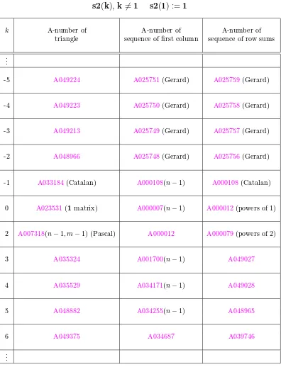
Table 1: Associated k-Stirling number triangles of the second kind
s2
(
k
),
k
6
=
1
s2
(
1
) :=
1
k A-number of A-number of A-number of
triangle sequence of first column sequence of row sums
.. .
-5 A049224 A025751(Gerard) A025759(Gerard)
-4 A049223 A025750(Gerard) A025758(Gerard)
-3 A049213 A025749(Gerard) A025757(Gerard)
-2 A048966 A025748(Gerard) A025756(Gerard)
-1 A033184(Catalan) A000108(n−1) A000108(Catalan)
0 A023531(1matrix) A000007(n−1) A000012(powers of 1)
2 A007318(n−1, m−1) (Pascal) A000012 A000079(powers of 2)
3 A035324 A001700(n−1) A049027
4 A035529 A034171(n−1) A049028
5 A048882 A034255(n−1) A048965
6 A049375 A034687 A039746
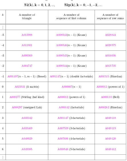
Table 2: k-Stirling number triangles of the second kind
S2
(
k
)
,
k
=
0
,
1
,
2
, ...,
S2p
(
k
)
,
k
=
0
,
−
1
,
−
2
, ...
k A-number of A-number of A-number of
triangle sequence of first column sequence of row sums
.. .
-5 A013988 A008543(n−1) (Keane) A028844
-4 A011801 A008546(n−1) (Keane) A028575
-3 A000369 A008545(n−1) (Keane) A016036
-2 A004747 A008544(n−1) (Keane) A015735
-1 A001497(n−1, m−1) (Bessel) A001147(n−1) (double factorials) A001515(Riordan)
0 A023531(1matrix) A000007(n−1) A000012(powers of 1)
1 A008277(Stirling 2nd kind) A000012(powers of 1) A000110(Bell)
2 A008297(unsigned Lah) A000142(factorials) A000262(Riordan)
3 A035342 A001147(2-factorials) A049118
4 A035469 A007559(3-factorials) A049119
5 A049029 A007696(4-factorials) A049120
6 A049385 A008548(5-factorials) A049412
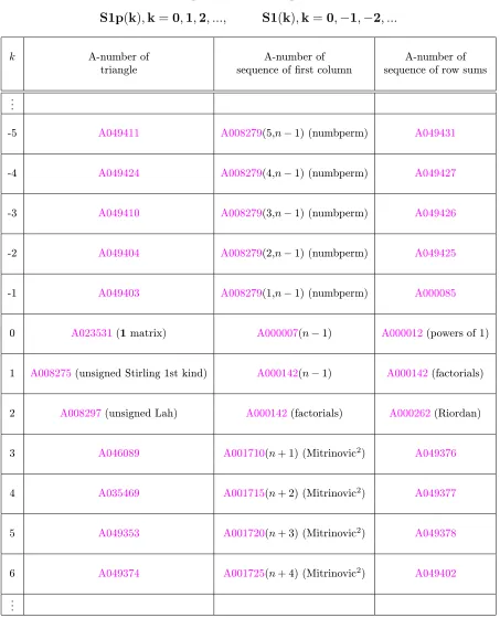
Table 3: Associated k-Stirling number triangles of the first kind
s1
(
k
),
k
6
=
1
s1
(
1
) :=
1
k A-number of A-number of A-number of
triangle sequence of first column sequence of row sums
.. .
-5 A049327 A049323(5,m) A049351
-4 A049326 A049323(4,m) A049350
-3 A049325 A049323(3,m) A049349
-2 A049324 A049323(2,m) A049348
-1 A030528 A019590=A049323(1, m) A000045(n+ 1) (Fibonacci)
0 A023531(1matrix) A000007(n−1)=A049323(0,m) A000012(powers of 1)
2 A007318(n−1, m−1) (Pascal) A000012(powers of 1) A000079(powers of 2)
3 A030523 A001792 A039717
4 A030524 A036068 A043553
5 A030526 A036070 A045624
6 A030527 A036083 A046088
Table 4: k-Stirling number triangles of the first kind
S1p
(
k
)
,
k
=
0
,
1
,
2
, ...,
S1
(
k
)
,
k
=
0
,
−
1
,
−
2
, ...
k A-number of A-number of A-number of
triangle sequence of first column sequence of row sums
.. .
-5 A049411 A008279(5,n−1) (numbperm) A049431
-4 A049424 A008279(4,n−1) (numbperm) A049427
-3 A049410 A008279(3,n−1) (numbperm) A049426
-2 A049404 A008279(2,n−1) (numbperm) A049425
-1 A049403 A008279(1,n−1) (numbperm) A000085
0 A023531(1matrix) A000007(n−1) A000012(powers of 1)
1 A008275(unsigned Stirling 1st kind) A000142(n−1) A000142(factorials)
2 A008297(unsigned Lah) A000142(factorials) A000262(Riordan)
3 A046089 A001710(n+ 1) (Mitrinovic2) A049376
4 A035469 A001715(n+ 2) (Mitrinovic2) A049377
5 A049353 A001720(n+ 3) (Mitrinovic2) A049378
6 A049374 A001725(n+ 4) (Mitrinovic2) A049402
(Concerned with sequencesA000007,A000012,A000045,A000079,A000085,A000108,A000110,A000142,A000262,
A000369,A001147,A001497,A001515,A001700,A001710,A001715,A001720,A001725,A001792,A004747,A007318,
A007559,A007696,A008275,A008277,A008279,A008297,A008543,A008544,A008545,A008546,A008548,A011801,
A013988,A015735,A016036,A019590,A023531,A025748,A025748-A025755,A025749,A025750,A025751,A025756,
A025757,A025758,A025759,A028575,A028844,A030523,A030524,A030526,A030527,A030528,A033184,A033842,
A034171,A034255,A034687,A035323,A035324,A035342,A035469,A035529,A036068,A036070,A036083,A039717,
A039746,A043553,A045624,A046088,A046089,A048882,A048965,A048966,A049027,A049028,A049029,A049118,
A049119,A049120,A049213,A049223,A049224,A049323,A049324,A049325,A049326,A049327,A049348,A049349,
A049350,A049351,A049353,A049374,A049375,A049376,A049377,A049378,A049385,A049402,A049403,A049404,
A049410,A049411,A049412,A049424,A049425,A049426,A049427,A049431,A053113.)
Received Feb. 11, 2000; published in Journal of Integer Sequences Sept. 13, 2000; minor editorial changes Nov. 30, 2000.