STRUCTURED CONDITIONING OF MATRIX FUNCTIONS∗ PHILIP I. DAVIES†
Abstract. The existing theory of conditioning for matrix functionsf(X):Cn×n→Cn×ndoes
not cater for structure in the matrixX. An extension of this theory is presented in which whenXhas structure, all perturbations ofX are required to have the same structure. Two classes of structured matrices are considered, those comprising the Jordan algebraJ and the Lie algebraLassociated with a nondegenerate bilinear or sesquilinear form on Rn or Cn. Examples of such classes are the symmetric, skew-symmetric, Hamiltonian and skew-Hamiltonian matrices. Structured condition numbers are defined for these two classes. Under certain conditions on the underlying scalar product, explicit representations are given for the structured condition numbers. Comparisons between the unstructured and structured condition numbers are then made. When the underlying scalar product is a sesquilinear form, it is shown that there is no difference between the values of the two condition numbers for (i) all functions ofX∈J, and (ii) odd and even functions ofX∈L. When the underlying scalar product is a bilinear form then equality is not guaranteed in all these cases. Where equality is not guaranteed, bounds are obtained for the ratio of the unstructured and structured condition numbers.
Key words. Matrix functions, Fr´echet derivative, Condition numbers, Bilinear forms,
Sesquilin-ear forms, Structured Matrices, Jordan algebra, Symmetric matrices, Lie algebra, Skew-symmetric matrices.
AMS subject classifications.15A57, 15A63, 65F30, 65F35.
1. Introduction. A theory of conditioning for matrix functions was developed by Kenney and Laub [6]. Condition numbers off(X)are obtained in terms of the norm of the Fr´echet derivative of the function atX. In this work a functionf(X)of a matrixX ∈Cn×n has the usual meaning, which can be defined in terms of a Cauchy integral formula, a Hermite interpolating polynomial, or the Jordan canonical form. It is assumed throughout that f is defined on the spectrum ofX. A large body of theory on matrix functions exists, with a comprehensive treatment available in [5].
In this work we extend the ideas of Kenney and Laub to structured matrices. That is, when X has structure then all perturbations of X are required to have the same structure. Enforcing structure on the perturbations enables the theory to respect the underlying physical problem. The structured matrices considered in this work arise in the context of nondegenerate bilinear or sesquilinear forms onRnorCn. This allows a wide variety of structured matrices to be considered. Examples of such classes of structured matrices are the symmetric, skew-symmetric, Hamiltonian and skew-Hamiltonian matrices.
In section 2 we review the original theory of conditioning of matrix functions [6] and discuss the unstructured condition number, K(f, X). In section 3 we briefly
∗Received by the editors 19 January, 2004. Accepted for publication 11 May, 2004. Handling
Editor: Ludwig Elsner. Numerical Analysis Report No. 441, Manchester Centre for Computational Mathematics, Manchester, England, Jan 2004.
†Department of Mathematics, University of Manchester, Manchester, M13 9PL, England
([email protected], http://www.maths.man.ac.uk/~ieuan). This work was supported by En-gineering and Physical Sciences Research Council grant GR/R22612.
review definitions and some relevant properties of bilinear forms,x, y=xTM yand sesquilinear formsx, y=x∗M y. We introduce some important classes of structured matrices associated with a bilinear or sesquilinear form. For two of these classes, the Jordan and Lie algebras, denoted by J and Lrespectively, we define structured condition numbers,KJ(f, X)andKL(f, X). Then, assuming thatM ∈Rn×n satisfies
M = ±MT and MTM = I, we give an explicit representation for these condition numbers. If the underlying scalar product is a bilinear form, then the structured condition numbers are equal to the 2-norm of a matrix. We then present an algorithm, based on the power method, for approximating these structured condition numbers. Numerical examples are given to show that after a few cycles of our algorithm, reliable estimates can be obtained.
In section 4, using the explicit representation of KJ(f, X), we compare the
un-structured and the un-structured condition number whenX ∈J. We first consider the case whereJis the Jordan algebra associated with a bilinear form. Experimental and theoretical evidence is used to show that KJ(f, X)and K(f, X)are often equal to
each other. However, examples can be found where the unstructured condition num-ber is larger than the structured condition numnum-ber. A bound forK(f, X)/KJ(f, X)
is then given which is linear in n. We then investigate the class of real symmetric matrices, which is the Jordan algebra associated with the bilinear formx, y=xTy. We show thatK(f, X) =KJ(f, X)for all symmetric X. We also show that whenJ
is the Jordan algebra associated with a sesquilinear form,K(f, X) =KJ(f, X)for all
X ∈J.
In section 5, using the explicit representation of KL(f, X), we compare the
un-structured and the un-structured condition number whenX ∈L. We first consider the case whereLis the Lie algebra associated with a bilinear form. For generalf, we have been unable to show anything about the relationship between the two condition num-bers. However, progress can be made if we restrictf to odd or even functions. For odd
f, we show that the ratio between the unstructured and the structured condition num-ber is unbounded. However, for evenf, we are able to show thatK(f, X) =KL(f, X)
for allX ∈L. We then investigate the class of real skew-symmetric matrices, which is the Lie algebra associated with the bilinear formx, y=xTy. For the exponential, cosine and sine functions we show that K(f, X) =KL(f, X)for all skew-symmetric
X. We then consider the case whereLis the Lie algebra associated with a sesquilinear form. We show thatK(f, X) =KL(f, X)for odd and even functionsf at allX∈L.
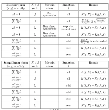
Finally, in section 6 we give our conclusions and some suggestions for future work. Table 6.1 gives a summary of the main results of this paper.
2. Conditioning of Matrix Functions. Using the theory developed by Ken-ney and Laub [6] we start by considering the effect of general perturbations ofX at
f. The functionf is Fr´echet differentiable atX if and only if there exists a bounded linear operatorL(·, X):Cn×n →Cn×n such that for allZ∈Cn×n whereZ= 1,
lim δ→0
f(X+δZ)−f(X)
δ −L(Z, X)
= 0.
The operator L is known as the Fr´echet derivative of f at X. The unstructured condition number of the matrix function is then defined using the Fr´echet derivative:
K(f, X) =L(·, X)F = max Z=0
L(Z, X)F
ZF .
(2.2)
Just as in [6], the Frobenius norm has been used because of its nice properties with respect to the Kronecker matrix product. The condition number defined in (2.2) relates the absolute errors of f at X. An alternative condition number is described in [1] that relates the relative errors off at X:
k(f, X) = L(·, X)FXF f(X)F
.
These two condition numbers are closely related:
k(f, X) =K(f, X) XF f(X)F
.
(2.3)
The focus of this paper shall be on the “absolute” condition number,K(f, X). Results for the “relative” condition number,k(f, X), can then be obtained using (2.3). We shall assume throughout thatf(X)can be expressed as a power series,
f(X) = ∞
m=0
αmXm, (2.4)
where αm ∈R and the equivalent scalar power seriesf(x) = ∞m=0αmxm is abso-lutely convergent for all |x| < r where X2 < r. This assumption encompasses a
wide range of functions, including functions such as the exponential, trigonometric and hyperbolic functions, whose Taylor series have an infinite radius of convergence. We shall also assume thatδ >0,Z2 ≤1 andX2+δ < r, so thatf(X+δZ)is
well defined in terms of the power series in (2.4). Then
f(X+δZ) =f(X) +δ
∞
m=1
αm m−1
k=0
XkZXm−1−k+O(δ2).
(2.5)
Using (2.5)together with (2.1), an explicit representation can be given for the Fr´echet derivative:
L(Z, X) = ∞
m=1
αm m−1
k=0
XkZXm−1−k.
Applying the vec operator (which forms a vector by stacking the columns of a matrix) toL(Z, X)and using the relation vec(AXB) = (BT ⊗A)vec(X) , we obtain
whereD(X)is the Kronecker form of the Fr´echet derivative:
D(X) = ∞
m=1
αm m−1
k=0
(XT)m−1−k⊗Xk. (2.6)
AsXF=vec(X)2 for allX, we have
K(f, X) = max Z=0
D(X)vec(Z)2 vec(Z)2
=D(X)2.
(2.7)
We shall now consider the effect on the condition number when structure is imposed onX and the perturbed matrixX+δZ.
3. Structured Matrices and Condition Numbers. In [8], Mackey, Mackey and Tisseur define classes of structured matrices that arise in the context of nonde-generate bilinear and sesquilinear forms. We shall briefly review the definitions and properties of such forms.
Consider a map (x, y)→ x, yfromKn×Kn toK, whereKdenotes the fieldR orC. If the map is linear in both argumentsxandy, that is,
α1x1+α2x2, y=α1x1, y+α2x2, y, x, β1y1+β2y2=β1x, y1+β2x, y2,
then this map is called a bilinear form. If K =C and the map x, y is conjugate linear in the first argument and linear in the second, that is,
α1x1+α2x2, y=α1∗x1, y+α∗2x2, y, x, β1y1+β2y2=β1x, y1+β2x, y2,
then this map is called a sesquilinear form.
For each bilinear form onKn, there exists a uniqueM ∈Kn×nsuch thatx, y= xTM y,∀x, y∈Kn. Similarly, for each sesquilinear form onCn, there exists a unique M ∈ Cn×n such thatx, y= x∗M y,∀x, y ∈Cn. A bilinear or sesquilinear form is nondegenerate if
x, y= 0, ∀y⇒x= 0,
x, y= 0, ∀x⇒y = 0.
It can be shown that a bilinear or sesquilinear form is nondegenerate if and only if
M is nonsingular. We shall use the term scalar product to refer to a nondegenerate bilinear or sesquilinear form onKn.
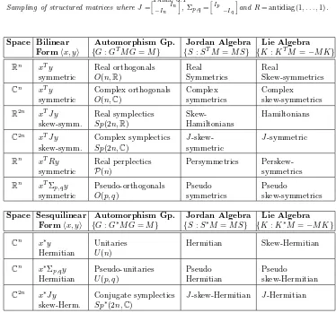
Table 3.1
Sampling of structured matrices whereJ=−I
n
In,Σ
p,q= I
p
−Iq
andR= antidiag(1, . . . ,1).
Space Bilinear Automorphism Gp. Jordan Algebra Lie Algebra Formx, y {G:GTM G=M} {S:STM =M S} {K:KTM=−M K}
Rn xTy Real orthogonals Real Real
symmetric O(n,R) Symmetrics Skew-symmetrics
Cn xTy Complex orthogonals Complex Complex symmetric O(n,C) symmetrics skew-symmetrics
R2n xTJy Real symplectics Skew- Hamiltonians skew-symm. Sp(2n,R) Hamiltonians
C2n xTJy Complex symplectics J-skew- J-symmetric skew-symm. Sp(2n,C) symmetric
Rn xTRy Real perplectics Persymmetrics
Perskew-symmetric P(n) symmetrics
Rn xTΣ
p,qy Pseudo-orthogonals Pseudo Pseudo
symmetric O(p, q) symmetrics skew-symmetrics
Space Sesquilinear Automorphism Gp. Jordan Algebra Lie Algebra Formx, y {G:G∗M G=M} {S:S∗M =M S} {K:K∗M =−M K}
Cn x∗y Unitaries Hermitian Skew-Hermitian Hermitian U(n)
Cn x∗Σ
p,qy Pseudo-unitaries Pseudo Pseudo
Hermitian U(p, q) Hermitian skew-Hermitian
C2n x∗Jy Conjugate symplectics J-skew-Hermitian J-Hermitian skew-Herm. Sp∗(2n,C)
Three important classes of structured matrices are associated with each scalar product.
1. The matricesGwhich preserve the value of the scalar product, that is,
Gx, Gy=x, y ∀x, y∈Kn.
The set G, known as the automorphism group of the scalar product, is thus defined as
Gdef= {G∈Kn×n:GTM G=M} for a bilinear form, Gdef= {G∈Cn×n:G∗M G=M} for a sesquilinear form.
2. The matricesS that areself-adjoint with respect to the scalar product, that is,
The setJ, known as the Jordan algebra related to the scalar product, is thus defined as
Jdef= {S∈Kn×n:STM =M S} for a bilinear form, Jdef= {S∈Cn×n:S∗M =M S} for a sesquilinear form.
3. The matrices K that are skew-adjoint with respect to the scalar product, that is,
Kx, y=−x, Ky ∀x, y∈Kn.
The set L, known as the Lie algebra related to the scalar product, is thus defined as
Ldef= {K∈Kn×n:KTM =−M K} for a bilinear form, Ldef= {K∈Cn×n:K∗M =−M K} for a sesquilinear form.
WhileGis a multiplicative group, it is not a linear subspace. However,Jand L do form linear subspaces. This means that if X and the perturbed matrixX +δZ
belong to J (or L), then the perturbation matrix Z must also belong to J (or L). Because of this linear property, the rest of this paper focuses only on matrices inJ andL. Table 3.1 shows some examples of well-known structured matrices associated with a scalar product.
The structured condition numbers are defined in a similar manner to the unstruc-tured condition number given in (2.2), except the perturbation matrixZ is restricted to eitherJorL. Therefore, we define
KJ(f, X) = max
Z=0,Z∈J
L(Z, X)F
ZF ,
KL(f, X) = max
Z=0,Z∈L
L(Z, X)F
ZF ,
whereL(Z, X)is defined in (2.1). Notice that no structure has been assumed on the matrixX. Imposing a similar structure onX will be considered in sections 4 and 5. We can also define “relative” structured condition numbers
kJ(f, X) =KJ(f, X) XF
f(X)F ,
kL(f, X) =KL(f, X) XF
f(X)F .
Notice that
k(f, X)
kJ(f, X)
= K(f, X)
KJ(f, X)
and k(f, X)
kL(f, X)
= K(f, X)
KL(f, X)
.
We shall now consider the structured condition numbers when the underlying scalar product is a bilinear form in section 3.1, and when the scalar product is a sesquilinear form in section 3.2.
3.1. Bilinear forms. In this section we shall assume that J and L denote a Jordan algebra and a Lie algebra associated with a nondegenerate bilinear form on Kn. ForS ∈J, it can be shown that vec(S)satisfies
(MT ⊗I)P−I⊗Mvec(S) = 0, (3.1)
where P is the vec-permutation matrix that satisfies Pvec(X)= vec(XT)for all X ∈Cn×n. From (3.1)we see that vec(S)is contained in the null space of (MT ⊗ I)P−I⊗M. Therefore the structured condition number off atX can be expressed as
KJ(f, X) = max
Z=0,Z∈J
D(X)vec(Z)2 vec(Z)2
=D(X)B2,
(3.2)
where the columns ofBform an orthonormal basis for the null space of (MT⊗I)P− I⊗M. ForK∈L, vec(K)satisfies
(MT⊗I)P+I⊗Mvec(K) = 0, and the structured condition number off at X can be given as
KL(f, X) = max
Z=0,Z∈L
D(X)vec(Z)2 vec(Z)2
=D(X)B2,
where the columns ofBform an orthonormal basis for the null space of (MT⊗I)P+ I⊗M. If M has certain properties, then more can be said about the null space of (MT ⊗I)P±I⊗M.
Lemma 3.1. LetM ∈Rn×n be nonsingular andM =δMT whereδ=±1. Define
SJ(M) = (MT ⊗I)P−I⊗M,
(3.3)
SL(M) = (MT ⊗I)P+I⊗M,
(3.4)
whereP is the vec-permutation matrix. Then
rank(SJ(M)) =n(n−δ)/2,
rank(SL(M)) =n(n+δ)/2.
Furthermore, if MTM =I, then the nonzero singular values of S
J(M) and SL(M) are equal to2.
Proof. Using the fact thatP(A⊗B) = (B⊗A)P for allA, B∈Cn×n [2] we can write
The vec-permutation matrixP is symmetric and has eigenvalues 1 and−1 with mul-tiplicities 1
2n(n+ 1) and 1
2n(n−1), respectively [2]. Since the matrixI⊗M has full
rank whenM is nonsingular,
rank(SJ(M) ) = rank(δP −I) =n(n−δ)/2.
A similar argument shows that rank(SL(M) ) = rank(δP+I) = 12n(n+δ).
WhenMTM =I the matrixI⊗M is orthogonal. Therefore, the matrixδP−I andSJ(M)have the same singular values. A similar argument shows thatδP+Iand
SL(M)have the same singular values.
Lemma 3.2. Let M ∈Rn×n be nonsingular andM =±MT. Then null(SJ(M)) = range(P SL(M)T),
null(SL(M)) = range(P SJ(M)T),
where P is the vec-permutation matrix and SJ(M), SL(M) are defined in (3.3) and
(3.4).
Proof. As a consequence of Lemma 3.1
dim(null(SJ(M))) = dim(range(P SL(M)T)),
dim(null(SL(M))) = dim(range(P SJ(M)T)),
and hence all we need to show is thatSJ(M)P SL(M)T = 0. Now
SJ(M)P SL(M)T = (MT⊗I)P(M ⊗I)−(I⊗M)P(I⊗MT) +
MT ⊗MT−M ⊗M.
AsM =±MT the third and fourth terms cancel. Further rearranging yields
SJ(M)P SL(M)T =P(M⊗MT)−P(M ⊗MT) = 0.
Theorem 3.3. Let X ∈ Cn×n and the scalar function f(x) = ∞
m=0αmxm
be absolutely convergent for all |x| < r where X2 < r. Also, let J and L denote a Jordan algebra and a Lie algebra associated with a nondegenerate bilinear form
x, y=xTM y, whereM ∈Rn×n satisfiesMTM =I andM =δMT where δ=±1.
Then
KJ(f, X) =
1
2D(X)P SL(M) T
2,
(3.5)
KL(f, X) =
1
2D(X)P SJ(M) T
2.
(3.6)
Proof. First, we considerZ ∈J. We have shown that vec(Z)∈null(SJ(M)) and
by Lemma 3.2 that vec(Z) ∈ range(P SL(M)T) . As MTM = I, Lemma 3.1 shows
that there exist orthogonal matricesU andV such that
P SL(M)T =U
2I
Letr= rank(P SL(M)T) = 12n(n+δ)and partition
U=
r n2−r
U1 U2
.
Then we can see that range(P SL(M)T)= range(U1)and U1TU1 =I. Therefore the
structured condition number off at X is
KJ(f, X) = max
Z=0,Z∈J.
D(X)vec(Z)2 vec(Z)2
=D(X)U12.
Define
B =
r n2−r
U1 0
=U
I
0 .
Then
KJ(f, X) =D(X)B2=
1
2D(X)P SL(M) TV
2,
=1
2D(X)P SL(M) T
2.
A similar argument can be used to give the result forKL(f, X).
In Theorem 3.3 we have assumed thatM =±MT andMTM =I. This may seem a restrictive condition. However, a wide variety of structured matrices are associated with bilinear forms that satisfy these conditions, including all those in Table 3.1.
By showing that SJ(M)SL(M)T = 0 when M =±MT and MTM =I, we can
show, using an almost identical proof of Lemma 3.2, that
null(SJ(M)) = range(SL(M)T),
null(SL(M)) = range(SJ(M)T).
Hence, using an almost identical proof of Theorem 3.3, we can show
KJ(f, X) =
1
2D(X)SL(M) T
2,
KL(f, X) =
1
2D(X)SJ(M) T
2.
We shall be using the forms (3.5)and (3.6)given in Theorem 3.3 as these involve less algebraic manipulation later.
3.1.1. Condition estimation. Kenney and Laub [6] presented a method for estimating the condition number K(f, X)by using the power method. The power method can be used to approximate A2 for a matrix A ∈ Cm×n. This method
fori= 1,2, . . .
z=z/z2, then computew=Az.
w=w/w2, then computez=ATw.
end
A2≈ z2
As long as the starting vector is not orthogonal to the singular subspace corresponding to the largest singular value ofA,z2converges toA2. The power method can then
be used to approximateD(X)2. As formingD(X)can be prohibitively expensive,
it is difficult to computeD(X)z0, wherez0= vec(Z0)for someZ0∈Cn×n. Therefore
we can use the “finite difference” relation
unvec(D(X)vec(Z0)) =
1
δ(f(X+δZ0)−f(X)) +O(δ)
(3.7)
where Z0F = 1. An approximation to D(X)vec(Z0) can be formed using a
suffi-ciently small δ. Starting with Z0F = 1, the two steps of the power method can then be approximated by
W = 1
δ(f(X+δZ0)−f(X)),
Z1= 1
δ
f(XT+δW
0)−f(XT),
where W0 = W/WF. ThenZ1F ≈ D(X)2. More accurate estimates can be
obtained by repeating the cycle withZ0=Z1/Z1F.
Now we consider how to estimate our structured condition numberKJ(f, X)by
using the power method to estimate 12D(X)P SL(M)T2. Starting withZ0 where Z0F = 1, lety= vec(Y) = 12P SL(M)Tvec(Z0).Then
Y =1 2
Z0MT +Z0TM
.
(3.8)
Letw= vec(W) =D(X)y. Then we can approximateW using
W ≈1
δ(f(X+δY)−f(X)).
The next stage is to scalewsuch that
w0= vec(W0) = vec(W/WF) =w/w2.
The final step is to computez1= vec(Z1) = 12(D(X)P SL(M)T)Tw0. Rearranging we
getz1= 12SL(M)P uwhere u= vec(U) =D(X)Tw0. Therefore we can approximate
U using
U ≈1
δ
f(XT +δW
0)−f(XT)
.
We can then formz1 by
Z1= 1
2
U M +M UT.
0 1000 2000 3000 4000 5000 6000 7000 8000 9000 10000 0.2
0.4 0.6 0.8 1 1.2
0 1000 2000 3000 4000 5000 6000 7000 8000 9000 10000
0.2 0.4 0.6 0.8 1 1.2
Fig. 3.1. Accuracy of estimates for structured condition numbers. (top) Mea-sures Kest
J (f, X)/KJ(f, X) for the 10000 examples in Experiment 4.2. (bottom) Measures Kest
L (f, X)/KL(f, X)for the 10000 examples in Experiment5.1.
Then Z1F ≈ 12D(X)P SL(M)T2. More accurate estimates can be obtained by
repeating the cycle withZ0=Z1/Z1F. To estimateKL(f, X) , we have exactly the
same procedure, except with the + sign in (3.8)and (3.9)changed to a−sign. Algorithm 3.4 (Estimation of structured condition numbers). Given X ∈
Kn×n and the scalar function f(x) =∞
m=0αmxm for which the series is absolutely
convergent for all|x|< rwhereX2< r, this algorithm computes an approximation to the condition numberKJ(f, X)or KL(f, X).
If we are computingKJ(f, X)thenk= 0. Otherwisek= 1.
Letδ= 100uXF where uis the unit roundoff. Computef(X).
Choose random nonzeroZ∈Kn×n. fori= 1,2, . . .
ifZF= 0, Z=Z/ZF, end Y =12(ZMT + (−1)kZTM). W =1δ(f(X+δY)−f(X)). ifWF = 0,W =W/WF, end U = 1δ(f(XT +δW)−f(X)T). Z =12(U M+ (−1)kM UT). end
Kest
In order to test whether Algorithm 3.4 produces reliable estimates to our struc-tured condition numbers we used random polynomials of random matrices inJorL, where J and L are the Jordan and Lie algebras relating to a bilinear form x, y =
xTM y, where M is a random symmetric orthogonal matrix. See Experiment 4.2, in section 4, and Experiment 5.1, in section 5, for more details on how this random data was produced. We used three cycles in Algorithm 3.4 to compute our esti-mates, Kest
J (f, X)and KLest(f, X). Figure 3.1 plots the ratios KJest(f, X)/KJ(f, X)
and Kest
L (f, X)/KL(f, X)for the 10000 examples in each experiment. We see from
Figure 3.1 that Algorithm 3.4 can overestimate the true condition number. This can be explained by the fact that approximations are used in some steps of the algorithm, for example (3.7). Also massive cancellation can occur in the computation of (3.7). However, in virtually all examples, the estimates are within a factor of 2 of the cor-rect value. As we are often only interested in the order of magnitude of the condition number, these results are acceptable.
An alternative to Algorithm 3.4 can be obtained by applying the power method to 12D(X)SL(M)T and 12D(X)SJ(M)T. Consider KJ(f, X)and the first step y =
vec(Y) = 12SL(M)Tvec(Z0) . Then
Y = 1 2(M Z
T
0 +MTZ0)
would replace the step (3.8). Then
W =1
δ(f(X+δY)−f(X)),
U =1
δ
f(XT +δW0)−f(XT),
whereW0=W/WF. We would also have to replace the final step (3.9)with
Z1=
1 2(U
TM+M U).
To estimate KL(f, X)we would again change the + signs to − signs in the
equa-tions for Y and Z1. No appreciable difference can be seen in practice between this
alternative algorithm and Algorithm 3.4.
3.2. Sesquilinear forms. In this section we shall assume thatJandLdenote a Jordan algebra and a Lie algebra associated with a nondegenerate sesquilinear form. ForS∈J, it can be shown that vec(S)satisfies
(MT ⊗I)vec(S∗)−(I⊗M)vec(S) = 0.
Provided M ∈ Rn×n then it can be shown that vec(Real(S)) ∈ null(S
J(M)) and
vec(Imag(S))∈null(SL(M)). Using Theorem 3.2 we can show that
vec(S) =P SL(M)Tx+iP SJ(M)Ty,
(3.10)
for somex, y ∈Rn2
.
Theorem 3.5. Let X ∈Cn×n and the scalar function f(x) =∞
m=0αmxm be
absolutely convergent for all |x| < r where X2 < r. Also, let J and L denote a Jordan algebra and a Lie algebra associated with a nondegenerate sesquilinear form
x, y=x∗M y, whereM ∈Rn×n satisfies MTM =I andM =δMT whereδ=±1.
Then
KJ(f, X) = max
v∈Cn2
D(X)(M⊗I)(v+δPv¯)2 (v+δPv¯)2 ,
(3.11)
KL(f, X) = max
v∈Cn2
D(X)(M⊗I)(v−δPv¯)2 (v−δPv¯)2
.
(3.12)
Proof. First we consider Z ∈ J. As M = δMT where δ = ±1 we can show, using (3.10), that
vec(Z) = (M⊗I)(v+δP¯v)
for some v ∈ Cn2. Substituting this into (3.2)and using the fact that M ⊗I is orthogonal whenM is orthogonal gives the result in (3.11). Using a similar argument we can show that forZ∈L,
vec(Z) = (M⊗I)(v−δPv¯)
for somev∈Cn2
and hence obtain the result in (3.12).
4. Jordan Algebra. In this section we shall compare the unstructured condi-tion number of f, K(f, X), with the structured condition number of f, KJ(f, X),
forX ∈J. We shall first consider the case where the underlying scalar product is a bilinear form. Then in section 4.2 we shall consider the case where the underlying scalar product is a sesquilinear form.
4.1. Bilinear forms. We shall first assume thatJ denotes the Jordan algebra relating to a nondegenerate bilinear formx, y=xTM ywhere M ∈ Rn×n satisfies M = δMT, δ = ±1 and MTM = I. Recall that (3.5)shows that the structured condition number off is equal to the 2-norm of the matrix 1
2D(X)P SL(M)T. As
pre-or post-multiplication by an pre-orthogonal matrix does not affect the singular values, we shall consider the matrix 12(I⊗M)D(X)P SL(M)T. It can be shown that
1
2(I⊗M)D(X)P SL(M) T = 1
2H(X)(In2+δP), (4.1)
where
H(X) = (I⊗M)D(X)(M ⊗I).
(4.2)
condition number, KJ(f, X), we shall compare the singular values of H(X)and 1
2H(X)(In2+δP).
WhenX ∈J, the matrixH(X)is highly structured. We can rearrangeH(X)to get:
H(X) = (I⊗M) ∞
m=1
αm m−1
k=0
(XT)m−1−k⊗Xk(M⊗I)
= (M ⊗M) ∞
m=1
αm m−1
k=0
Xm−1−k⊗Xk.
(4.3)
From (4.3)it is easy to see that: • H(X) =H(X)T.
• H(X)commutes withP, that isP H(X) =H(X)P.
• H(X) = ([H(X)]ij)is a blockn×nmatrix where each block satisfies
[H(X)]ij=δ[H(X)]Tij ∈Kn×n.
The following result about matrices that commute with unitary matrices allows us to compare the singular values ofH(X)and 1
2H(X)(In2+δP).
Lemma 4.1. Let A, B∈Cn×n, whereB is a Hermitian unitary matrix, satisfy
AB=±BA.
Let B have eigenvalues 1 with multiplicity p and −1 with multiplicity n−p. Then 1
2A(I+B) has psingular values in common with A andn−pzero singular values. Also 1
2A(I−B) has the other n−p singular values in common with A plus pzero singular values.
Proof. We can write the singular value decomposition ofA asA=UΣV∗ where Σ is partitioned in block diagonal form such that Σ = diag(σjI)whereσ1>· · ·> σk are thekdistinct singular values ofA. IfAB=±BA, then (UΣV∗)B=±B(UΣV∗) and
Σ =±(U∗BU)Σ(V∗BV)∗.
(4.4)
As B is unitary, this is just a singular value decomposition of a diagonal matrix. ThereforeU∗BU andV∗BV must be block diagonal matrices and conformably par-titioned with Σ [5, Theorem 3.1.1′]. Using this, we can see that
1
2A(I+B) = 1
2U(Σ(I+V
∗BV))V∗
=Udiagσj
2 (I+Ej)
V∗
where E = V∗BV = diag(E
j) . As B is Hermitian, the block diagonal matrix diagσj
2(I+Ej)
is also Hermitian. Therefore the singular values of 1
2A(I+B)are
equal to the absolute values of the eigenvalues of diagσj
2(I+Ej)
has eigenvalues±1 and hence so do the diagonal blocksEj. LetEjhave eigenvalues 1 with multiplicitypjand−1 with multiplicitynj. Then the diagonal block σ2j(I+Ej) hasσj as an eigenvalue with multiplicitypj and 0 as an eigenvalue with multiplicity nj. Askj=1pj =p, 12A(I+B)haspsingular values in common withA. A similar argument shows that
1
2A(I−B) =Udiag
σj
2 (I−Ej)
V∗
and therefore 12A(I−B)has the othern−psingular values ofAthat are “missing” from 12A(I+B) .
Using Lemma 4.1 we can see that 12H(X)(In2+δP)has 12n(n+δ)singular values
in common withH(X). The natural question arises: which singular values ofH(X) does 12H(X)(In2 +δP)share and do they have the same largest singular value? To
gain insight into this question we performed the following experiment 10000 times. Experiment 4.2. Using normally distributed random variables with mean 0 and variance 1, generate
• Random Householder matrixM such thatM y=y2e1wherey is a random vector in R3.
• Random polynomialf(x) =a6x6+· · ·+a1x+a0 where the coefficientsai are
randomly distributed.
• Random X ∈ J. This is formed using random A∈R3×3 and forming X =
AMT +ATM.
Using this data, H(X)is formed, from which the condition numbers K(f, X) and KJ(f, X)are computed. In all 10000 examples we found K(f, X) =KJ(f, X).
This seemed to suggest that equality may hold for allf, M where M =±MT and MTM =I, andX ∈J. However, examples whereK(f, X)> K
J(f, X)can be found.
For example, take
• Householder matrixM such thatM y=y2e1where
y= [−0.4442 −0.5578 −0.2641 ]T.
• A polynomial
f(x) =−0.2879x6+ 1.2611x5+ 2.3149x4−0.2079x3+ 2.1715x2+ 0.6125x.
• X =AMT +ATM ∈Jwhere
A=
−−20..08201035 −00.1206.1532 −10.4778.7404 1.0344 1.1157 −0.9895
.
In this example, K(f, X) = 10.5813 while KJ(f, X) = 8.7644. This example was
generated using direct search methods in MATLAB to try to maximize the ratio
K(f, X)/KJ(f, X). The ratio in this example is just over 1.2073, which suggests that
Examples where K(f, X) > KJ(f, X)seem very rare and hard to characterize.
However, for the class of real symmetric matrices, which is the Jordan algebra relating to the bilinear formx, y=xTy, we show in section 4.1.3 thatK(f, X) =K
J(f, X)
for all symmetricX.
4.1.1.. What about the other singular values of H(X)? To see what hap-pened to the singular values ofH(X)that are not singular values of1
2H(X)(In2+δP),
consider the condition number off atX, whereX∈J, subject to perturbations from the Lie algebra:
KL(f, X) =
1
2(I⊗M)D(X)P SJ(M) T
2.
It is easily seen that
1
2(I⊗M)D(X)P SJ(M) T = 1
2H(X)(In2−δP),
whereH(X)is defined in (4.2). Using Lemma 4.1 we can see that 12H(X)(In2−δP)
has the other 12n(n−δ)singular values ofH(X)that are “missing” from 12H(X)(In2+
δP). This also shows that whenX ∈J,
K(f, X) = max{KJ(f, X), KL(f, X)}.
4.1.2. Bounding K(f, X)/KJ(f, X). In order to bound the ratio of the
un-structured and un-structured condition numbers, where X ∈ J, we shall consider the set
H={H∈Kn2×n2:H = (Hij)withHij =δHijT ∈Kn×n andP H=HP}, (4.5)
whereδ=±1 andP is the vec-permutation matrix. All possibleH(X) , formed from a functionf atX ∈J, belong toH. Therefore
max X∈J
K(f, X)
KJ(f, X) ≤max
G∈H
2G2 G(In2+δP)2
.
The interesting case is whereH(X)2>12H(X)(In2+δP)2. We have shown that
when this happensH(X)2= 12H(X)(In2−δP)2. Therefore we can equivalently
consider
max G∈H
G(In2−δP)2 G(In2+δP)2
.
In order to exploit the properties of the matrices inHit is convenient to introduce a 4-point coordinate system to identify elements ofG∈H:
Therefore (a, b, c, d)refers to the element ofGin thebth row of theath block row and thedth column of thecth block column. We can now interpret the two properties of H:
(a, b, c, d) =δ(a, d, c, b)(regardingGij =δGTij), (4.6)
(a, b, c, d) = (b, a, d, c)(regardingGP =P G).
(4.7)
Using an alternate application of (4.6)and (4.7)we can show that
(a, b, c, d) = δ(a, d, c, b) =
δ(d, a, b, c) = (d, c, b, a) = (c, d, a, b) = δ(c, b, a, d) =
δ(b, c, d, a) = (b, a, d, c).
(4.8)
It can be seen from (4.8)that (a, b, c, d) = (c, d, a, b)and therefore Gis symmetric. Also noticeable is the fact that the left hand side of (4.8)are all the cyclic permutations of (a, b, c, d)while the right hand side of (4.8)are all the cyclic permutations of the reverse ordering (d, c, b, a). Other permutations ofa, b, canddgive different elements ofG:
(a, b, d, c) = δ(a, c, d, b) =
δ(c, a, b, d) = (c, d, b, a) = (d, c, a, b) = δ(d, b, a, c) =
δ(b, d, c, a) = (b, a, c, d),
(4.9)
and
(a, c, b, d) = δ(a, d, b, c) =
δ(d, a, c, b) = (d, b, c, a) = (b, d, a, c) = δ(b, c, a, d) =
δ(c, b, d, a) = (c, a, d, b).
(4.10)
All 4! permutations of a, b, c and d are accounted for. When a, b, c and d are all distinct integers then we have three sets of eight elements where all elements in the same set have the same value (up to signs). However, when a, b, cand dare not all distinct integers then all the elements will be repeated the same number of times in the lists (4.8), (4.9) and (4.10). Also, the integers a, b, cand d won’t refer to three unique values of G. For example, whena=b,a, b, c and drefer to just two unique values ofG. This is seen from the fact that list (4.8)is identical to the list (4.9)and the list (4.10)only refers to four unique elements ofG.
Lemma 4.3. Let Hbe as defined in(4.5). Then
max G∈H
G(In2 −δP)2 G(In2 +δP)2
≤
3n(n+δ)
2 ,
Proof. We can first show that
max G∈H
G(In2−δP)2 G(In2+δP)2 ≤maxG∈H
rank(G(In2+δP))
G(In2−δP)F
G(In2+δP)F
≤
n(n+δ) 2 maxG∈H
G(In2−δP)F
G(In2+δP)F .
Now we have to bound maxG∈H G
(In2−δP) F
G(In2+δP) F. Define the ordered set
S={{a, b, c, d}: 1≤a≤b≤c≤d≤n}
and
T{a,b,c,d}={{p, q, r, s}: All distinct permutations of{a, b, c, d} ∈S}.
As (GP)n(a−1)+b,n(c−1)+d= (a, b, d, c),
G(In2−δP)2F
G(In2+δP)2F
=
{a,b,c,d}∈Sf(a, b, c, d)
{a,b,c,d}∈Sg(a, b, c, d)
where
f(a, b, c, d) = {p,q,r,s}∈T{a,b,c,d}
((p, q, r, s)−δ(p, q, s, r))2,
g(a, b, c, d) = {p,q,r,s}∈T{a,b,c,d}
((p, q, r, s) +δ(p, q, s, r))2.
It can easily be shown that
max G∈H
G(In2−δP)2F
G(In2+δP)2F
≤ max {a,b,c,d}∈S
maxf(a, b, c, d)
g(a, b, c, d)
.
Now we have to bound maxfg((a,b,c,da,b,c,d)) for all possible{a, b, c, d} ∈S.
All a, b, c and d different. Letx= (a, b, c, d), y = (a, c, d, b)andz = (a, d, b, c). Then we can show that for all{a, b, c, d} ∈S,
f(a, b, c, d)
g(a, b, c, d) =
8(x−y)2+ (y−z)2+ (z−x)2
8 ((x+y)2+ (y+z)2+ (z+x)2).
(4.11)
Rearranging yields
f(a, b, c, d)
g(a, b, c, d) =
3(x2+y2+z2)−(x+y+z)2
(x2+y2+z2) + (x+y+z)2
Two integers equal, two different. Let x = (a, a, c, d), y = (a, c, d, a) , and z = (a, d, a, c) . Forδ= 1, it is easy to see from (4.8)and (4.9)thatx=y. Then,
f(a, a, c, d) = 8(x−z)2, g(a, a, c, d) = 8(x+z)2+ 16x2.
Notice that fg((a,a,c,da,a,c,d)) is a special case of (4.11)where x = y and therefore has a maximum of 3 at 2x+z= 0. Forδ=−1,
f(a, a, c, d) = 24x2, g(a, a, c, d) = 8x2.
This is also a special case of (4.11)wherex=−y andz= 0 (z= (d, a, c, a)which is on the diagonal of a block)and fg((a,a,c,da,a,c,d)) is always the maximum 3.
Two integers equal twice. Letx= (a, a, d, d), y= (a, d, d, a) , and z= (a, d, a, d). Forδ= 1,x=y and
f(a, a, d, d) = 4(x−z)2, g(a, a, d, d) = 4(x+z)2+ 8x2.
Therefore maxfg((a,a,d,da,a,d,d))= 3 at 2x+z= 0. Forδ=−1,x=−y,z= 0 and
f(a, a, d, d) = 12x2, g(a, a, d, d) = 4x2,
and fg((a,a,d,da,a,d,d))= 3.
More than two integers equal. Let x = (a, a, a, d), y = (a, a, d, a) , and z = (a, d, a, a) . For δ = 1, it can be shown that x = y = z. This means, all permu-tations of (a, a, a, d)are equal. Hencef(a, a, a, d)= 0 and maxfg((a,a,a,da,a,a,d)) = 0 for all
x, y andz. Forδ=−1, we havex=y=z= 0 and thereforef(a, a, a, d) = 0. Therefore max{a,b,c,d}∈S(maxf
(a,b,c,d)
g(a,b,c,d))= 3 and the result follows immediately
from this.
Theorem 4.4. Let X ∈ J, where J denotes the Jordan algebra relating to a nondegenerate bilinear form x, y= xTM y, where M ∈Rn×n satisfies MTM =I
andM =δMT for δ=±1. Let the scalar function
f(x) = ∞
m=0
αmxm
be absolutely convergent for all |x|< rwhereX2< r. Then
K(f, X)
KJ(f, X) ≤
3n(n+δ)
2 .
4.1.3. Real symmetric case (M =I). It is known that restricting perturba-tions to symmetric linear systems or eigenvalue problems to be symmetric makes little difference to the backward error or the condition of the problem [3], [4]. The same can be shown for the condition of matrix functions. We shall start with the following lemma, which is essentially the same as a result given in [6, Lemma 2.1], but written as a matrix factorization.
Lemma 4.5. Let X ∈ Rn×n be diagonalizable and have the eigendecomposition X =QDQ−1whereD= diag(λ
k). Then the Kronecker form of the Fr´echet derivative
off(X)is also diagonalizable and has the eigendecompositionD(X) =VΦV−1 where
V =Q−T ⊗Q,Φ = diag(φ k)and
φn(i−1)+j =
f(λi)−f(λ
j)
λi−λj λi=λj,
f′(λ
j) λi=λj.
Proof. Considering Φ =V−1D(X)V, we see that
Φ = ∞
m=1
αm m−1
k=0
Dm−1−k⊗Dk = diag(φ k).
Thekth diagonal element of Φ, wherek=n(i−1)+j for some unique 1≤i, j ≤n, is then given by
φk =
∞
m=1
αm m−1
k=0
λmi −1−kλk j.
Ifλi =λj, including the case wherei=j, thenmk=0−1λ
m−1−k
i λkj =mλ m−1
i and
φk=
∞
m=1
αmmλmi −1=f
′(λ
i).
Ifλi =λj, then
m−1
k=0 λmi −1−kλkj = λm
i −λ m j
λi−λj and
φk =
∞
m=1
αm λm
i −λmj λi−λj
=f(λi)−f(λj)
λi−λj .
We now consider a symmetric matrixX and the condition number off atX, subject to symmetric perturbations.
Theorem 4.6. LetX =XT ∈Rn×nand the scalar functionf(x) =∞
m=0αmxm
be absolutely convergent for all |x|< rwhereX2< r. Then
Proof. We have seen thatK(f, X) =D(X)2 and Theorem 3.3 shows that
KJ(f, X) = max
Z=0,Zsymm.
L(Z, X)F
ZF
=1
2D(X)P SL(I) T
2.
Therefore, we shall compare the singular values ofD(X)and1
2D(X)P SL(I)T to show
our result. AsM =Iwe can see thatD(X) =H(X) , whereH(X)is defined in (4.2), and from (4.1), 1
2D(X)P SL(I)T = 1
2H(X)(In2+δP)and therefore both matrices are
symmetric.
AsX is symmetric, we can write its eigendecompositionX =QDQT whereQis orthogonal andD= diag(λk). ¿From Lemma 4.5 we see thatD(X) =VΦVT where V =Q⊗Qis also orthogonal and Φ = diag(φk). It is easy to see that P commutes withV, and therefore
1
2D(X)P SL(I) T =1
2V(ΦP+ Φ)V T.
As φn(i−1)+j =φn(j−1)+i, a similarity transformation can be applied to 12(ΦP + Φ)
using a permutation matrix to get a block diagonal matrix consisting of • n1×1 blocks [φn(i−1)+i] for 1≤i≤n.
• 1
2n(n−1)2×2 blocks 1 2
φ φ φ φ
whereφ=φn(i−1)+j for 1≤i < j≤n. Hence the eigenvaluesµk of 12(ΦP+ Φ) are
µn(i−1)+j=
φn(i−1)+j i≤j, 0 i > j.
The nonzero parts of the spectra ofD(X)and 1
2D(X)P SL(I)T are equal, if
multiplic-ities are ignored. As both matrices are symmetric, their singular values are equal to the absolute values of their eigenvalues and so D(X)2=12D(X)P SL(I)T2.
Theorem 4.6 shows that the condition number of f at a symmetric matrix X is unaffected if the perturbations are restricted to just symmetric perturbations.
4.2. Sesquilinear forms. We shall now assume that J denotes the Jordan al-gebra relating to a nondegenerate sesquilinear formx, y=x∗M ywhereM ∈Rn×n satisfiesM =δMT,δ=±1 andMTM =I. From (3.11)we can show that
KJ(f, X) = max
v∈Cn2
H(X)(v+δPv¯)2 v+δP¯v2
,
whereH(X)is defined in (4.2). WhenX ∈J, the matrixH(X)is highly structured and it can be shown that
• H(X)is Hermitian. • H(X)P =P H(X)T.
Using these properties ofH(X)we can obtain the following result.
Lemma 4.7. LetH ∈Rn2×n2 satisfy HP =P HT andH =µH∗ whereµ=±1. Then
max v∈Cn2
H(v+αP¯v)2 v+αPv¯2
whereα∈C.
Proof. Consider an eigenpair (λ, y)of H. If H is Hermitian, its eigenvalues are real. IfH is skew-Hermitian, its eigenvalues are purely imaginary. Therefore
H(y+αPy¯) =Hy+αP HTy,¯ =λy+αP(µλ¯y¯),
=λ(y+αPy¯).
Ify+αPy¯= 0, then we can always replaceywithβywhereβ ∈Cand Imag(β)= 0. Theny+αPy¯is an eigenvector ofH corresponding to the eigenvalueλ. AsH =±H∗, its singular values are equal to the absolute values of its eigenvalues. Therefore, using the eigenvectorsyk ofH, we have
σk =
H(yk+αPy¯k)2 yk+αPy¯k2
for all singular valuesσk ofH. The result follows immediately from this.
Theorem 4.8. Let X ∈ J, where J denotes the Jordan algebra relating to a nondegenerate sesquilinear formx, y=x∗M y, whereM ∈Rn×nsatisfiesMTM =I
andM =δMT for δ=±1. Let the scalar function
f(x) = ∞
m=0
αmxm
be absolutely convergent for all |x|< rwhereX2< r. Then
K(f, X) =KJ(f, X).
Proof. This result comes easily from Lemma 4.7 usingα=δ.
We can also show that
KL(f, X) = max
v∈Cn2
H(X)(v−δP¯v)2 v−δPv¯2 .
Therefore using Lemma 4.7 withα=−δwe can also show thatK(f, X) =KL(f, X)
under the same conditions onf,X andJ that are used in Theorem 4.8.
5. Lie Algebra. In this section we shall compare the unstructured condition number of f, K(f, X), with the structured condition number of f, KL(f, X) , for
5.1. Bilinear forms. We shall first assume thatLdenotes the Lie algebra re-lating to a nondegenerate bilinear form x, y = xTM y where M ∈ Rn×n satisfies M =δMT, δ=±1 andMTM =I. To compare the unstructured condition number K(f, X), with the structured condition numberKL(f, X), we shall compare the
sin-gular values of D(X)and those of 1
2D(X)P SJ(M)T. Equivalently, we can compare
the singular values of H(X), defined in (4.2), and 1
2H(X)(In2 −δP) . We have not
been able to find a pattern between these singular values. For an arbitrary function
f(X)andX ∈L, the matrixH(X)is not necessarily symmetric nor does it commute withP. However, iff is restricted to being an odd or even function, then a pattern arises. This is a natural restriction, as f is an odd function if and only iff(L)⊆L, whilef is an even function if and only iff(L)⊆J[7].
First, consider an odd function f(X) = ∞m=0α2m+1X2m+1. The Kronecker
form of the Fr´echet derivative off is
D(X) = ∞
m=1
α2m−1 2m−2
k=0
(XT)2m−2−k⊗Xk.
WhenX ∈L, the matrixH(X)is highly structured. We can rearrangeH(X)to get:
H(X) = (I⊗M)D(X)(M⊗I),
= (M ⊗M) ∞
m=1
α2m−1 2m−2
k=0
(−1)kX2m−2−k⊗Xk.
It can be shown that • H(X) =H(X)T.
• H(X)commutes withP, that isP H(X) =H(X)P.
Using Lemma 4.1 we can show that the matrix12H(X)(In2−δP)has12n(n−δ)singular
values in common withH(X). The natural question arises: which singular values of
H(X)does 12H(X)(In2−δP)share and do they have the same largest singular values?
To gain insight into this question we performed the following experiment 10000 times. Experiment 5.1. Using normally distributed random variables with mean 0 and variance 1, generate
• Random Householder matrixM such thatM y=y2e1wherey is a random vector in R3.
• Random polynomial f(x) =a5x5+a3x3+a1x where the coefficients ai are
randomly distributed.
• Random X ∈L. This is formed using random A∈R3×3 and forming X =
AMT −ATM.
Using this data, H(X)is formed, from which the condition numbers K(f, X) and KL(f, X)are computed. We found a marked difference between the results of
Experiment 4.2 and 5.1. Out of 10000 examples, on just 740 occasions did we find
K(f, X) = KL(f, X) . Also K(f, X)/KL(f, X)could grow large. In this experiment
we achieved a maximum ofK(f, X)/KL(f, X)= 349. In fact, this ratio is unbounded.
Let
X =
0 1
whereLis the Lie algebra associated with the bilinear formx, y=xTy, that is, the class of skew-symmetric matrices. Letf(X) =X3+ 3X. Then
H(X) =
1 0 0 −1
0 1 1 0
0 1 1 0
−1 0 0 1
.
Note that H(X)P is the same as H(X)except that the second and third columns have been swapped over. Then, it is easy to see that 1
2H(X)(In2 −δP) = 0 and
thereforeKL(f, X)= 0. Hence,K(f, X)/KL(f, X)is unbounded at X. We can call
X a “stationary point” of the functionf(X) =X3+ 3X whenX is restricted to the
class of skew-symmetric matrices.
Now, consider an even functionf(X) =∞m=0α2mX2m. The Kronecker form of the Fr´echet derivative off is
D(X) = ∞
m=1
α2m
2m−1
k=0
(XT)2m−1−k⊗Xk.
WhenX ∈L, the matrixH(X)is highly structured. We can rearrangeH(X)to get:
H(X) = (I⊗M)D(X)(M⊗I),
= (M⊗M) ∞
m=1
α2m
2m−1
k=0
(−1)k+1X2m−1−k⊗Xk.
It can be shown that • H(X) =−H(X)T.
• H(X)also satisfiesP H(X) =−H(X)P.
These conditions are more restrictive on the singular values of H(X)than those for odd functions. Because of this, more can be said about the structured condition number at evenf.
Theorem 5.2. Let X ∈L, where L denotes the Lie algebra relating to a non-degenerate bilinear form x, y=xTM y, where M ∈Rn×n satisfies M =±MT and MTM =I. Let the even scalar function
f(x) = ∞
m=0
α2mx2m
be absolutely convergent for all |x|< rwhereX2< r. Then
K(f, X) =KL(f, X).
Proof. We have shown thatK(f, X) =H(X)2 and
KL(f, X) =
1
Therefore, we shall compare the singular values of H(X)and 1
2H(X)(In2−δP)to
show our result. Define
M(X) = 1
2H(X)(In2−P),
N(X) = 1
2H(X)(In2+P).
When X ∈ L and f is an even function, it can be shown that M(X) = −N(X)T. ThereforeM(X)andN(X)have the same singular values. Using Lemma 4.1 we can show thatM(X)has 12n(n−1)singular values in common withH(X)(plus 12n(n+ 1) zero singular values)whileN(X)has the other 12n(n+ 1)singular values of H(X) (plus 1
2n(n−1)zero singular values). As we have shown M(X)andN(X)have the
same singular values, then
H(X)2=M(X)2=N(X)2.
Recall that
KJ(f, X) =
1
2H(X)(In2+δP)2
whereδ=±1. Therefore, the proof of Theorem 5.2 also shows that forX ∈Land an even functionf, the condition number is unaffected if the perturbations are restricted toJ. That isK(f, X) =KJ(f, X).
5.1.1. Real skew-symmetric case (M =I). We now compare the unstruc-tured and the strucunstruc-tured condition numbers off atX when X is a skew-symmetric matrix. We have seen that K(f, X) =D(X)2 and Theorem 3.3 shows that
KL(f, X) = max
Z=0,Zskew.
L(Z, X)F
ZF
=1
2D(X)P SJ(I) T
2.
Therefore, we shall compare the singular values ofD(X)and12D(X)P SJ(I)T. Using a
slightly modified version of Lemma 4.5, whereXT is replaced byX∗in the Kronecker form of the Fr´echet derivative, we can show that if X has the eigendecomposition
X =QDQ∗ whereQis unitary andD= diag(λ
i)thenD(X) =VΦV∗ where
Φ = ∞
m=1
αm m−1
k=0
(D∗)m−1−k⊗Dk= diag(φk)
andV =Q⊗Q. The diagonal elements of Φ are given by
φn(i−1)+j=
f(λ∗
i)−f(λj)
λ∗
i−λj λ
∗
i =λj, f′(λ
j) λ∗i =λj. (5.1)
AsP commutes withV, it is easy to see that
1
2D(X)P SJ(I) T = 1
By applying a similarity transformation to 1
2(ΦP −Φ)using a permutation matrix
we can get a block diagonal matrix consisting ofn 1×1 blocks whose elements are zero and 1
2n(n−1)2×2 blocks
Λij = 1 2
−φn(i−1)+j φn(j−1)+i φn(i−1)+j −φn(j−1)+i
for 1≤i < j ≤n. Using the fact thatf(λ∗
k) = f(λk)∗, it is easy to see from (5.1) that φn(i−1)+j =φ∗n(j−1)+i. Therefore the singular values of Λij are|φn(i−1)+j| and 0 and the singular values of 12(ΦP−Φ)are
σn(i−1)+j=
0 i≤j
|φn(i−1)+j| i > j. (5.2)
As in the symmetric case, the singular values of D(X)exist in pairs, |φn(i−1)+j| =
|φn(j−1)+i|. However, ignoring multiplicities, not all the nonzero singular values of D(X)appear as singular values of 12D(X)P SJ(I)T. The “missing” singular values
are
σi=|φn(i−1)+i|=
|f(λ∗i)−f(λi)
λ∗
i−λi | λi = 0, |f′(0)| λ
i = 0. (5.3)
For certain functions these “missing” singular values are never the largest singular values of D(X)and so, for these functions, we have K(f, X) = KL(f, X)for all
skew-symmetricX.
Lemma 5.3. Let the scalar functionf(x) =∞m=0αmxmbe absolutely convergent
for all|x|< r, and let
max
|f′(0)|,
f(µi)−f(−µi) 2µ
≤ |f′(µi)|.
(5.4)
for all realµ such that 0<|µ|< r. Then
K(f, X) =KL(f, X)
for all skew-symmetricX such that0<X2< r.
Proof. A skew-symmetric matrix has purely imaginary eigenvalues which we denote byλk =iµk. Then using (5.3)we see that
σk =
|f(−iµk)2µ−f(iµk)
k | λk= 0, |f′(0)| λ
k= 0.
are the singular values of D(X)that are not singular values of 12D(X)P SJ(I)T.
All we have to show is that, providing (5.4)holds, there exists a singular value of
1
AsX is a real matrix, its eigenvalues exist in complex conjugate pairs. Therefore, for each nonzero eigenvalueλi, then λi=λ∗j for somej. From (5.1), we can see that
|φn(i−1)+j|=|f′(λj)| and |φn(j−1)+i|=|f′(λi)|
are singular values of D(X), and from (5.2), we can see that one of them is also a singular value of 1
2D(X)P SJ(I)
T. As |f′(λ
i)| = |f′(λj)|, we can use (5.4)to show there exists a singular value of 12D(X)P SJ(I)T greater than or equal to maxσk.
The condition (5.4)in Lemma 5.3 holds when f is a wide range of functions, including exponential, sine, cosine and cosh. For cosine and cosh and other even functions, this result has already been proved in Theorem 5.2. It can also be seen that the left hand side of (5.4)is zero for even functions. However this condition (5.4)does not hold for sinh. Examples whereK(sinh, X)> KL(sinh, X)are easily generated.
5.1.2. Skew-symmetric case, symmetric perturbations. If we consider the condition number off atX, whereX is skew-symmetric, subject to symmetric per-turbations, then Theorem 3.3 shows that
KJ(f, X) = max
Z=0,Zsymm.
L(Z, X)F
ZF
=1
2D(X)P SL(I) T
2.
It is easy to see that
1
2D(X)P SL(I) T = 1
2V(ΦP+ Φ)V ∗,
and the singular values of 1
2(ΦP+ Φ) are
σn(i−1)+j =
|φn(i−1)+j| i≤j 0 i > j.
As |φn(i−1)+j| = |φn(j−1)+i| for all 1 ≤ i, j ≤ n, all the nonzero singular values of D(X)appear as singular values of 12D(X)P SL(I)T, if multiplicities are ignored.
Therefore K(f, X) = KJ(f, X)which means the condition number of f at a
skew-symmetricX, is unaffected if the perturbations are restricted to just symmetric per-turbations.
5.2. Sesquilinear forms. We shall now assume thatLdenotes the Lie algebra relating to a nondegenerate sesquilinear formx, y=x∗M ywhereM ∈Rn×nsatisfies M =δMT,δ=±1 andMTM =I. From (3.12)we can show that
KL(f, X) = max
v∈Cn2
H(X)(v−δP¯v)2 v−δPv¯2
,
whereH(X)is defined in (4.2). We shall again restrict our attention to odd or even functions ofX, as this gives properties ofH(X)which we can work with. For an odd functionf(x) =∞m=0α2m+1x2m+1 andX ∈L, we can show that
• H(X)P=P H(X)T.
For an even functionf(x) =∞m=0α2mx2mandX ∈L, we can show that
• H(X)is skew-Hermitian. • H(X)P=P H(X)T.
These properties enable us to prove the following result.
Theorem 5.4. Let X ∈L, whereLdenotes the Lie algebra relating to a nonde-generate sesquilinear form x, y=x∗M ywhere M ∈Rn×n satisfiesMTM =I and M =δMT for δ=±1. Let thef(x)be either
• An odd scalar functionfodd(x) =∞m=0α2m+1x2m+1. • An even scalar functionfeven(x) =m∞=0α2mx2m.
Also, letf(x)be absolutely convergent for all |x|< r whereX2< r. Then
K(f, X) =KL(f, X).
Proof. This result comes from the fact that H(X)satisfies the conditions of Lemma 4.7 for both functionsfodd(x)andfeven(x).
Using Lemma 4.7 withα=δwe can also show that K(f, X) =KJ(f, X)under
the same conditions onf,X andLthat are used in Theorem 5.4.
6. Concluding Remarks. Kenney and Laub [6] presented a theory of condi-tioning of matrix functions f(X) based on the Fr´echet derivative at X. We have extended this theory by imposing structure onX and its perturbations. Structured conditioned numbers have been defined and, under certain conditions on the underly-ing scalar products, explicit representations have been given for them in Theorem 3.3 and Theorem 3.5. Comparisons between the unstructured and the structured condi-tion numbers were made and Table 6.1 summarizes the main results of this paper. If the underlying scalar product is a sesquilinear form, we have shown that imposing structure does not affect the condition number off for
• All functionsf ofX∈J.
• Odd or even functionsf ofX∈L.
However, when the underlying scalar product is a bilinear form, equality between the two condition numbers is not guaranteed in these cases. For generalf and X ∈ J, we have provided experimental and theoretical evidence to show thatKJ(f, X)and
K(f, X)are often equal to each other. However, equality does not always hold and a bound
K(f, X)
KJ(f, X)
<
3n(n+δ) 2 (6.1)
was proved. A few questions merit further investigation:
• Is it possible to characterize whenK(f, X) =KJ(f, X)?
• We have not been able to construct examples where the left hand side of (6.1) is much larger than 1.2. Are better bounds obtainable? Or, can we generate examples where KK(f,X)
Bilinear form X∈J Matrix Function Result
x, y=xTM y orL class f
M =I J symmetricsReal all K(f, X) =KJ(f, X)
MTM=I
M=±MT J all
K(f,X)
KJ(f,X) ≤
3n(n+δ) 2
M =I L symmetricsReal skew- exp, sin,
cos and cosh K(f, X) =KL(f, X)
M =I L symmetricsReal skew- all K(f, X) =KJ(f, X)
MTM=I
M=±MT L odd
K(f,X)
KL(f,X) is unbounded MTM=I
M=±MT L even K(f, X) =KL(f, X)
MTM=I
M=±MT L even K(f, X) =KJ(f, X)
Sesquilinear form X∈J Matrix Function Result
x, y=x∗M y orL class f
MTM=I
M=±MT J all K(f, X) =KJ(f, X)
MTM=I
M=±MT J all K(f, X) =KL(f, X)
MTM=I
M=±MT L odd K(f, X) =KL(f, X)
MTM=I
M=±MT L odd K(f, X) =KJ(f, X)
MTM=I
M=±MT L even K(f, X) =KL(f, X)
MTM=I
[image:29.595.110.471.142.507.2]M=±MT L even K(f, X) =KJ(f, X)
Table 6.1
Summary of main results comparing unstructured and structured condition numbers. “all” means all functions that can be written as a convergent power series.
For generalf and X ∈L less is known. The matrix H(X)has no observably nice properties to work with. A natural restriction is to consider odd and even functions ofX ∈L. For evenf we have shown thatK(f, X) =KL(f, X) . For oddf, the ratio
K(f, X)/KL(f, X)is unbounded. More information aboutf,X andLis required to
form more meaningful bounds on this ratio.
REFERENCES
[1] I. Gohberg and I. Koltracht. Condition numbers for functions of matrices. Appl. Numer. Math., 12(1-3):107–117, 1993.
[2] Harold V. Henderson and S. R. Searle. The vec-permutation matrix, the vec operator and Kronecker products: A review.Linear and Multilinear Algebra, 9(4):271–288, 1980/81. [3] Desmond J. Higham and Nicholas J. Higham. Backward error and condition of structured linear
systems. SIAM J. Matrix Anal. Appl., 13(1):162–175, 1992.
[4] Desmond J. Higham and Nicholas J. Higham. Structured backward error and condition of generalized eigenvalue problems. SIAM J. Matrix Anal. Appl., 20(2):493–512, 1998. [5] Roger A. Horn and Charles R. Johnson.Topics in Matrix Analysis. Cambridge University Press,
Cambridge, 1994. Corrected reprint of the 1991 original.
[6] Charles Kenney and Alan J. Laub. Condition estimates for matrix functions. SIAM J. Matrix Anal. Appl., 10(2):191–209, 1989.
[7] D. Steven Mackey. Private communication, December 2003.