Beta random fractions of a size-biased sample
Geurt Jongbloed
Delft Institute of Applied Mathematics
Delft University of Technology
The Netherlands
November 15, 2012
1
Introduction
two opposing mechanisms (selected interval tends to be longer than usual, but only part of its length is the actual waiting time) cancel. This cancelation is specific for the Poisson process; more general renewal processes do not share this property.
In section 2, the relation between the distribution of a random fraction from a biased draw from a distribution will be derived. The relation is specialized to the situation where the biasing happens proportional to a specific measure of size and the random fractions have a Beta distribution. Section 3 contains classical as well as more recent examples of the general problem.
2
The general problem
Consider a distribution function F on (0,∞) and a weight function w : [0,∞) → [0,∞) such that
0<
Z
w(x)dF(x)<∞.
The w-biased distribution associated to F has distribution function
F(w)(x) = 1 wF
Z x
0 w(y)dF(y), wherewF =
Z ∞
0 w(y)dF(y).
For weight functionw(x) = x, the distributionw-biased distribution is known as thelength biased distribution.
Now consider the second mechanism. Suppose X ≥ 0 has distribution function G, Y ≥0 has probability density k and X and Y are independent. Then, defining for z > 0 the set Cz = {(x, y) ∈ IR+2 : y ≤ z/x} the random variable Z = XY has distribution function
GZ(z) = P(XY ≤z) =P ((X, Y)∈Cz) =
Z ∞
y=0
Z z/y
x=0 k(x)dG(y)dx
=
Z ∞
y=0
Z z
x=0 1 yk
x y
!
dx dG(y) =
Z z
x=0
Z ∞
y=0 1 yk
x y
!
dG(y)dx
with density
gZ(z) =
Z ∞
y=0 1 yk
z y
!
dG(y)
If the random variable Y takes values in (0,1), this boils down to
gZ(z) =
Z ∞
y=z
1 yk
z y
!
dG(y)
Specializing even more, to Y having a B(α, β) distribution, so
k(y) = y
α−1(1−y)β−1
we obtain the following density of the product Z:
gZ(z) =
zα−1 B(α, β)
Z ∞
y=zy
α−β−1(y−z)β−1dG(y).
In combining the two mechanisms, we assume G to be a biased version of distribution function F. More specifically, for γ ∈IRwe assume that
G(z) = 1 wF,γ
Z z
0 y
γdF(y) with w F,γ =
Z ∞
0 y
γdF(y).
Then the distribution of the observableZ can be written as
gZ(z) =
zα−1 B(α, β)wF,γ
Z ∞
y=zy
α−β+γ−1(y
−z)β−1dF(y).
In section 3 we will see that some well known statistical models fit within the framework of estimating a distribution function F based on a sample of Beta random fractions of a ‘size-biased’ sample fromF, where ‘size’ is measured as a power of the variable of interest: Xγ. Moreover, the Beta distributions all come from the branch with α= 1.
3
Specific instances of the model
In this section we consider three models that fit within the framework of section 2. For the first two examples, the basic setting is identical. In an opaque medium, ball centers are distributed according to a (low intensity) homogeneous Poisson process and the corre-sponding squared ball radii all have the same distribution functionF. Moreover, these are independent. One is interested in the distribution of the (squared) ball radii, but direct observations on the radii are not obtainable. In example 3.1, data are obtained by inter-secting the medium with a line and observing the traces of the balls on the line. In example 3.2, the medium is cut by a plane and (circular) profiles of the balls on the intersecting plane are observed.
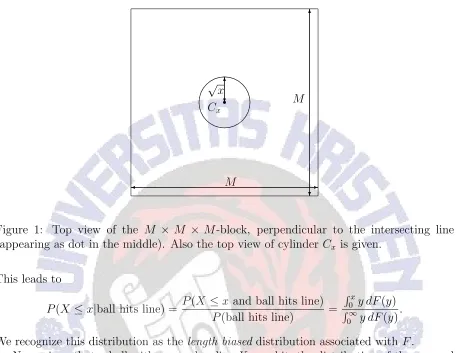
Example 3.1 (Linear probe problem). This model was described in [8]. Let us derive the distribution of the squared radius of a ball given that it is hit by the line. Think of a large block of sizeM×M×M and assume for simplicity that the radii of the balls do not exceed the valueM/2. Figure 1 gives the top-view of this block. Suppose the line intersects the block perpendicular to the plane in Figure 1, right at the middle (see the dot). Now, given the squared radius of a ball equals x, what is the probability that the (fixed) line intersects this ball when its center is placed uniformly at random within the block? This event occurs if and only if the center of the ball is placed in the circular cylinder with the intersecting line as axis, with radius√x. Denote this cylinder by Cx. Because the location
of the center is taken uniformly over the opaque block, we have
P(ball hits line|X =x) = volume of cylinder Cx volume of block =
M πx
M3 =
. . . . ... . . ... . . . . ... . . ... . ... ... ... . ... ... ... ... . . ... . ... ... . . ... ... . . . . . . . . . . . . . . . . . . . . . . . . . . . . . . . . . . . . . . . . . . . . . . . . . . . . . . . . . . . . . . . . . . . . . . . . . . . . . . . . . . . . . . . . . . . . . .
. . . . . . . . . . . . . . . ...
. . . . . . . . . . . . . . . . . . . . . . . . . . . . . . . . . . . . . . . . . . . . . . . . . . . . . . . . . . . . . . . . . . . . . . . . . . . . . . . . . . . . . . . . . . . . . .
r ✻ ❄
√x
Cx
✻
❄
M
✲
✛ M
Figure 1: Top view of the M × M × M-block, perpendicular to the intersecting line (appearing as dot in the middle). Also the top view of cylinder Cx is given.
This leads to
P(X≤x|ball hits line) = P(X ≤x and ball hits line) P(ball hits line) =
Rx
0 y dF(y)
R∞
0 y dF(y) .
We recognize this distribution as the length biased distribution associated with F.
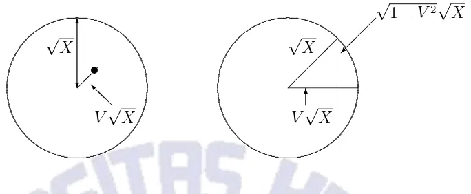
Now, given that a ball with squared radius X was hit, the distribution of the squared half-length of the trace of this ball on the line can be derived from the picture in Figure 2. The top view shows the contour of the ball of radius √X. Uniformly at random on this contour, the line intersects the ball. The dot indicates this position. The (perpendicular) distance of the ball center to the intersecting line is given by V√X, where for 0≤v ≤1
P(V ≤v) = area of circle with radius v area of circle with radius one =v
2.
From the right picture in Figure 2 we see that the observed squared half-length of the line segment intersecting the ball is given by
Z =X(1−V2) = ZY
where Y is a random variable, independent of X, and for 0≤y≤1
P(Y ≤y) =P(V2 ≥1−y) =P(V ≥q1−y) =y.
.
Figure 2: The left picture shows the top-view of an intersected ball of radius √X. The point indicates the (uniformly at random chosen) position where the line transects the ball. The distance of the ball center to the intersecting line is V√X. The right picture shows the same ball, but now from the direction perpendicular to the plane spanned by the ball center and the intersecting line. The ‘squared half-length’ of the observable line segment is given by (1−V2)X.
of this observation. This leads to the following sampling density for the observed squared half-length of the trace:
g(z) = 1
Note that the inverse relation can be easily obtained from this expression. Indeed,
1−F(z) = g(z) g(0).
This means that estimating F at a point z entails estimating the bounded decreasing densityg atz as well as at 0. Estimation ofg is usually done using the maximum likelihood estimator, also known as Grenander estimator ([1]). This estimator has good asymptotic properties on intervals [ǫ,∞), but is inconsistent at zero. See e.g. [10] for a discussion on this inconsistency as well as a penalization approach that can be adopted to consistently estimate g(0).
It is clear that the linear probe problem is related to the waiting time paradox described in the introduction. Note that an exponential distribution function F corresponds to the same exponential sampling density, as remarked in the introduction. Indeed, for x≥0
F(x) = 1−e−θx
⇐⇒ g(z) =θe−θx.
✲ ✛
√x
Sx
✻
❄
M
✲
✛ M
Figure 3: Top view of the M × M × M-block, perpendicular to the intersecting line (appearing as dashed line in the middle). Also the top view of slice Sx is given.
Putting the ball center in the block will now only give a nonempty intersection with the cutting plane if the center is put in the slice Sx depicted in Figure 3. We therefore get
P(ball hits plane|X =x) = volume of sliceSx volume of block =
2M2√x
M3 =
2√x
M .
This leads to
P(X ≤x|ball hits plane) = P(X ≤x and ball hits plane) P(ball hits plane) =
Rx
0 √y dF(y)
R∞
0 √y dF(y) .
We recognize this distribution as the weighted distribution associated withF with weight function w(x) =√x.
As illustrated in Figure 4, given a sphere with squared radius X is cut, the observable squared radius of the observable circle can be expressed as (1 −U2)X for U standard uniformly distributed and independent of X. This means that Wicksell’s problem fits within the framework of section 2 with γ = β = 1/2 and α = 1. Indeed, the sampling density g can be expressed in terms of F:
g(z) =
R∞
z (y−z)−1/2dF(y)
2R∞
0 √y dF(y) The inverse relation is given by
1−F(z) =
R∞
z (y−z)−1/2g(y)dy
R∞
.
cutting plane
✻ ❄
√
Z =√1−U2√X
Figure 4: View on the sphere in the direction of the vertical cutting plane. The sphere radius is √X, the position of the cut is uniformly distributed on the right half of the sphere.
Example 3.3 (Hampel problem). Consider a population of birds of a certain type that cross the desert individually and stop over at an oasis. Ornithologists are interested in the time spent by a generic bird at this oasis. The following model can be used to investigate these sojourn times. This problem was first described in [4].
To each bird, a positive random variable X with distribution function F is attached, denoting the time spent at the oasis. This quantity cannot be observed. Also, independent of X, the bird has a homogeneous Poisson process (N(t))t≥0 attached to it, with intensity λ, assumed to be small. The times the bird is caught at the oasis are then those jump points of the Poisson process that occur during the interval [0, X]. Note thatN(X) is the number of times the bird is caught.
The data for one bird consists of those catching times that occurred before X. Of course, conditional on the fact thatN(X)≥1. In Hampel’s model only those observations are used that correspond to birds that have been caught exactly twice. We will derive the distribution of the difference in time between the two catches in terms of the unknown distribution functionX of the sojourn time.
The first question is: what is the distribution of the sojourn time of a bird given it is caught exactly twice?
P(X ≤x|N(X) = 2) = P(X ≤x∧N(X) = 2)
for smallλ (and, for example, if F has bounded support). In other words, the conditional distribution is (for smallλ) the weighted distribution associated withF with weightw(x) = x2.
for the order statistics of two uniformly distributed random variables in (0,1)
P(Z > z|X =x) =P(U(2)−U(1) > z/x) = (1−z/x)2 for 0< z < x.
Consequently,
P(Z > z) =
Z ∞
0 P(Z > z|X =x)d ˜ F(x) =
R∞
z (x−z)2dF(x)
R∞
0 x2dF(x)
. (1)
We see that we explicitly have to require the second moment ofF to exist. However, if we take F to have bounded support, this assumption certainly holds.
Differentiating (1) with respect to z, we get for the densityg of Z that
g(z) = 2
R∞
z (x−z)dF(x)
R∞
0 x2dF(x) and differentiating once again gives
g′
(z) = −R2(1∞ −F(z))
0 x2dF(x)
This shows that the density g is necessarily convex and decreasing on (0,∞). Moreover, the inverse relation expressing F in terms ofg is given by
F(z) = 1− g
′(z)
g′(0)
The problem of estimatingF boils down to estimating the derivative of a convex decreasing densityg. In particular, estimating F(z) for z >0 entails estimation of the derivative of g atz and 0. This problem was studied thoroughly in [3].
4
Discussion
In this note we derive the relation between an underlying distribution functionF and the density of a random variable that is obtained from a two-step procedure. This procedure entails drawing a biased observation fromF and taking an (independent) random fraction of this draw, where the fraction has a beta distribution. This gives a whole family of inverse problems, where one can study the problem of estimating F based on a sample from density g.
References
[1] Grenander, U. (1957). On the theory of mortality measurement. II. Skand. Aktuari-etidskr., 39, p. 125-153.
[2] Groeneboom, P. and Jongbloed, G. (1995). Isotonic estimation and rates of conver-gence in Wicksell’s problem. The Annals of Statistics 23, p. 1518-1542.
[3] Groeneboom, P., Jongbloed, G. and Wellner, J.A. (2001). Estimation of a convex function: characterizations and asymptotic theory. The Annals of Statistics 29, p. 1653-1698.
[4] Hampel, F.R. (1987). Design, modelling and analysis of some biological datasets. In C.L. Mallows, editor, Design, data and analysis, by some friends of Cuthbert Daniel, p. 111-115, Wiley, New York.
[5] McGarrity, K.S., Sietsma, J. and Jongbloed, G. (2012). Nonparametric inference in a stereological model with oriented cylinders applied to dual phase steel. Submitted.
[6] Ross, S.M. (2010).Introduction to Probability Models,10-th edition. Elsevier, Amster-dam.
[7] Sen, B. and Woodroofe, M. (2012). Bootstrap Confidence Intervals for Isotonic Esti-mators in a Stereological Problem. To appear in Bernoulli.
[8] Watson, G.S. (1971). Estimating functionals of particle size distributions. Biometrika 58, p. 483-490.
[9] Wicksell, S.D. (1925). The corpuscle problem. Biometrika17, p. 84-99.