PREDICTION OF WIND SPEEDS BASED ON DIGITAL ELEVATION MODELS USING
BOOSTED REGRESSION TREES
Peter Fischera,∗, Christophe Etienneb, Jiaojiao Tiana, Thomas Kraußa
a
Remote Sensing Technology Institute, German Aerospace Center (DLR), M¨unchener Str. 20, 82234 Wessling, Germany -(Peter.Fischer, Jiaojiao.Tian, Thomas.Krauss)@dlr.de
b
Secquaero Advisors Ltd., 8001 Z¨urich, Switzerland - [email protected]
Commission VI, WG I/5
KEY WORDS:Digital Elevation Model, Wind Speed, Non-Parametric Regression
ABSTRACT:
In this paper a new approach is presented to predict maximum wind speeds using Gradient Boosted Regression Trees (GBRT). GBRT are a non-parametric regression technique used in various applications, suitable to make predictions without having an in-depth a-priori knowledge about the functional dependancies between the predictors and the response variables. Our aim is to predict maximum wind speeds based on predictors, which are derived from a digital elevation model (DEM). The predictors describe the orography of the Area-of-Interest (AoI) by various means like first and second order derivatives of the DEM, but also higher sophisticated classifications describing exposure and shelterness of the terrain to wind flux. In order to take the different scales into account which probably influence the streams and turbulences of wind flow over complex terrain, the predictors are computed on different spatial resolutions ranging from 30 m up to 2000 m. The geographic area used for examination of the approach is Switzerland, a mountainious region in the heart of europe, dominated by the alps, but also covering large valleys. The full workflow is described in this paper, which consists of data preparation using image processing techniques, model training using a state-of-the-art machine learning algorithm, in-depth analysis of the trained model, validation of the model and application of the model to generate a wind speed map.
1. INTRODUCTION
The strong linkage between geomorphologic parameters and wind flux has been used to describe a broad range of phenomena in-fluenced and driven by wind, like estimating the direction of an unknown air pollution source (Antoni´c and Legovi´c, 1999), map-ping wind erosion risk and dust emission-deposition (Reiche et al., 2012) or simulating snow redistribution and accumulation (Winstral and Marks, 2002). Besides of ecologic applications, the discrete description of wind flux and maximum wind speeds is also a key parameter to estimate the risk of damages by wind, Heneka (Heneka and Ruck, 2004) gives a detailed overview of different loss functions based on maximum wind speeds.
Estimating wind speeds over complex terrain is a challenging task, thus different methodical approaches exist to make such predictions. The domain of meteorological models deals with atmospheric boundary layers and the description of interactions in the atmosphere to model the behaviour of airflows, detailed application examples are given in (Hofherr and Kunz, 2010) and (de Rooy and Kok, 2004). Using Computational Fluid Dynam-ics (CFD) programs who solve the discrete Navier-Stokes equa-tion are also suitable for simulating wind speeds, but preparing such a simulation and running it is very resource demanding from a computational point of view. The DEM needs to be trans-formed into a volumetric mesh which represents the surface and the boundary conditions of the simulation in a sufficient manner, otherwise the air mass transportation would give no reliable re-sults. Garcia and Boulanger (Garcia and Boulanger, n.d.) give an example in using a CFD program for simulating low altitude wind flow, using a SRTM dataset with an spatial extent of more than 10000km2, covering Mt. St. Helens (USA).
∗Corresponding author. Tel.: +49 8153 281561; Fax: +49 8153
281444.
Besides of these strict mechanical models which aim to simu-late air flow, also general statistic techniques can be adapted for making spatial predictions, different tools are found in the regres-sion domain. The goal of regresregres-sion analysis is to uncover func-tional dependancies between a set of independent parameters and a set of dependent variables. By using such techniques, it’s pos-sible to make quantitative predictions with a known uncertainty based on a set of random samples. As the strict functional model is quite complex for wind speed prediction, it seems beneficial to use techniques from the non-parametric regression domain. Lehmann (Lehmann et al., 2002b) developed a software pack-age called Generalized Regression Analysis and Spatial Predic-tions (GRASP), which uses generalized additive models (GAMs) to modell the spatial behavour of a broad range of phenomena. It has been successfully used for different applications in ecolog-ical modelling, keywords are vegetation mapping, biodiversity and spatial species distributions (Cawsey et al., 2002, Lehmann et al., 2002a, Overton et al., 2002, Ray et al., 2002, Zaniewski et al., 2002). Besides of GAMs, also other non-parametric re-gression methods have been used for making spatial predictions. Leathwick (Leathwick et al., 2005) gave an example in using multivariate adaptive regression splines (MARS) to predict the occurance and density of fish populations in New Zealand fresh-water system. They used a broad range of environmental vari-ables like stream size, temperature and distance from the sea, the probabilites of occurance were then used to produce maps for New Zealands entire river network. A working guide to boosted regression trees (BRTs) is given by Elith (Elith et al., 2008), the use case is deals also with the distribution of a fish species in New Zealands river network.
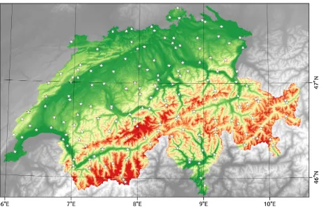
Figure 1: Wheather stations of MeteoSwiss
visualized as tree, which makes the model easy to understand and interpret. Introduced by Breiman (Breiman et al., 1984), over the last decades a broad range of extensions was developed. An in-depth description of the algorithm with practical examples is given in (Hastie et al., 2001). Boosting is an extension of the initial regression tree algorithm. Instead of creating a single tree, boosting creates iteratively an ensemble of trees which aim to minimize the residuals of the initial model. The final model con-sists of a collection of trees, following a gradient-descent strat-egy, where different loss functions (Mean Square Error, Absolute Error, Huber Loss, etc. ) are possible.
As the prediction of the wind speed strongly relies on the earth surface, a set of describing parameters is derived from the initial DEM. Besides of first and second order derivatives like slope, aspect and curvature, also a geomorphologic classification algo-rithm for landform analysis is used. Introduced by Weiss (Weiss, 2001), the Terrain Positioning Index (TPI) distinguishes between major landforms (hills, ridges, valley and others), which have an impact on the near ground air mass transportation system. An additional wind specific index based on DEM which provides a numerical measure of the degree of wind shelter, the TOPEX score, is also taken into account. A discussion of the TOPEX score and other qualitative and quantitative methods to assess topographic exposure is given by Chapman (Chapman, 2000). Both TPI and TOPEX have in common that they give freedom to the user about the maximum distance of height values to take into account, which helps to adjust the algorithm to the specific application.
2. AREA OF INTEREST, DATA
The study site is Switzerland, a mountainous region in the heart of Europe. The diversified landscape includes mountains higher than 4000 meters and steep canyons, but also farm land, lakes
and urban areas. The southern part of switzerland is dominated by the alps, leading to a dynamic orography with more than 3000 mountains higher than 2000 meters. The DEM was recorded by the SRTM mission and is provided with a spatial resolution of 30 meters (Farr et al., 2007). Having a representative set of wind measurements is essential for the task. The Federal Office of Me-teorology and Climatology MeteoSwiss maintains a network of more than 200 weather stations. The data are conveniently acces-sible via the online portal IDAweb at no charge for research. An overview of the locations of the weather stations is given in fig-ure 1, the height of the stations ranges from 203 to 3580 meters above sea level (asl).
2.1 WHEATHER STATIONS
The 200 weather stations used for this work are fully automatic and deliver wind speed and wind directions at an interval of 10 minutes. The station situated at the lowest altitude of 203 m asl is placed in Magadino/Cadenazzo. The place is part of the can-ton Tessin, and is less than 10 km from the famous lake Garda. The highest station is placed at the Jungfernjoch in the canton of Bern, at an altitude of 3580 m asl. The Jungfernjoch is a sad-dle between the two mountains Jungfrau and M¨onch, having the famous mountain Eiger nearby. The average altitude of all sta-tions is about 1032 m asl. The gust peak measuremens (one sec-ond) are delivered in a day-wise granularity, the time span taken into account starts in January 1981 and ends in September 2015. From the listed measurements for each station the 98th percentile (W98) was derived and then used for the evaluation.
2.2 PREDICTOR VARIABLES
(a) DEM, color encoding from black to white (min. to max. height) (b) TOPEX, color encoding from white to blue (min. to max. angle score)
Figure 2: Comparison of DEM (left) and derived TOPEX map (right)
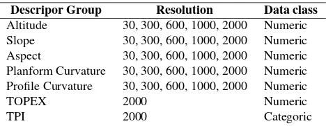
and 2000 m. For each DEM, the first and second order deriva-tives slope, aspect, profile and plan curvature were calculated. An detailed description of the derivatives is given by Wilson and Gallant (Wilson and Gallant, 2000). The landform classification is based on the TPI using two kernel maps, one with 100 m inner radius and 500 m outer radius, one with 100 m inner radius and 2000 m outer radius. In combination with a slope map a clas-sification into 10 major landforms is done, the classes are like suggested by Weiss (Weiss, 2001). The TOPEX score map is calculated taking the height values in a range from 100 m to 2000 m in the eight major cardinal directions into account. Figure 2 shows a subset of the DEM and the corresponding TOPEX map. An overview about the at least 7 different predictor groups and the different scales is given in table 1.
As all predictors rely on the DEM and several predictors are avail-able at different scales, orthogonality between the single predic-tors becomes an issue. On the one hand, one descriptor at dif-ferent scales could be useful to simulate difdif-ferent channelling and deflection effects of wind flow, on the other hand introduc-ing several correlated predictors into the model buildintroduc-ing process will blow up the model without increasing the overall accuracy. To overcome this problem, minimum one and maximum two de-scriptors of each of the descriptor groups is used for the final modelling. In the single descriptor groups the goal is to choose the two predictors having the lowest Pearson correlation coeffi-cient, as a restriction the correlation coefficient between variables of one group must not exceed 0.75. This approach enforces to add all relevant information to the model building process with-out overwhelming it with a big group of orthogonal predictors.
Descripor Group Resolution Data class
Altitude 30, 300, 600, 1000, 2000 Numeric
Slope 30, 300, 600, 1000, 2000 Numeric
Aspect 30, 300, 600, 1000, 2000 Numeric Planform Curvature 30, 300, 600, 1000, 2000 Numeric Profile Curvature 30, 300, 600, 1000, 2000 Numeric
TOPEX 2000 Numeric
TPI 2000 Categoric
Table 1: Description of Stock Data attributes
3. METHODOLOGY
GBRTs is considered as an ensemble method, combining sev-eral weak learners to a strong predictor. The term regression tree names already the type of learner. Regression Trees are known
for their simplicity in interpretation, for being able to handle nu-merical and categorical data, and for being able to fit complex non-linear relationships and interactions between predictors. In this examination for each geo-referenced wind measurementya set of predictor variables is derived from the DEM, denoted byx. A regression tree is then an estimatefˆof the functional depen-dancy between the predictorsxand the responsey.
Regression trees aim to partition the feature space into piecewise constant functions, also refered as regions. The description of such a functional model by a single tree is given in equation 1. In the final model each predictorxis linked to a regionR, the lim-iting borders ofRare defined by the intervalI.Mis the number of regions which corresponds to the number of split points of the tree plus one (having binary split points) andccorresponds to the constant response value predicted by the model. The building of a single tree is an iterative process, at each node the predictor variable and its value are chosen in order to minimize the over-all error of the model. Depending on the nature of the problem different loss functions can be used, like sum of squares, Huber loss or others. The response value is than the average value of all response values satisfying the rule set given by the tree.
ˆ
f(x) = M
X
m=1
cmI(x∈Rm) (1)
Gradient Boosting means that instead of growing one single re-gression tree, several trees are modelled and added to a model, where each new tree aims to minimize the residuals of the exist-ing model. Equation 2 describes this process, where the model Fm(x)at boosting stepmconsists of the modelFm−1(x)plus the regression treefˆ, which aims to minimize the residuals of Fm−1(x). In most algorithm implemetations the number of trees of the final model has to be specified by the user, but also a stop-ping criterion would be possible.
Fm(x) =Fm−1(x) + ˆf(x) (2)
re-As predictor for the final model, the DEM with 30 m spatial res-olution was used. All down sampled versions had a correlation coefficient higher than 0.8 to each other, therefore they would not add any further information. From the slope maps the resolution combination of 30 m and 1000 m has the lowest correlation coef-ficient with 0.49, for the aspect maps the combination 30 m and 600 m resulted in the minimum correlation coefficient of 0.13. For both profile and plan curvature the combination of 30 m and 2000 m spatial resolution give the lowest correlation coefficient nearby zero. The TOPEX map and the TPI map are taken as is.
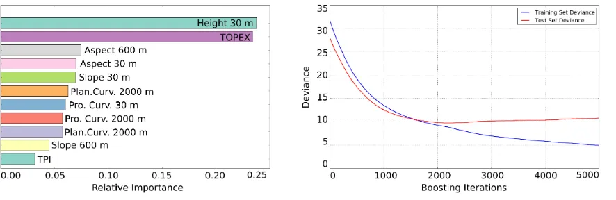
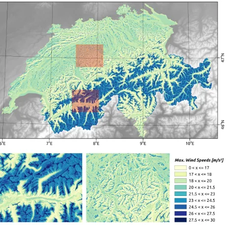
Figure 3(a) gives an overview of the influence of the single pre-dictors in the final model. As expected, altitude and TOPEX are the two predictors who contribute most to the final model. As mountain peaks and ridges are in most cases not sheltered by higher topographic entities in their neighbourhood, the influence of this parameter seams obvious. Figure 4 shows the maximum Wind Speed map, here we also see the strong influence of the altitude, as the underlying landforms are clearly visible. Areas which are sheltered by surrounding entities can easily be distin-guished from unsheltered areas by the TOPEX score. Areas hav-ing a high TOPEX score are less exposed to wind streams than areas in open valleys, because of this we expect the lowest wind speeds in such sheltered areas. The wind speed map proves this, as the lowest wind speeds are measured and also predicted in the submontane regions. Lakes have a TOPEX score nearby zero, the large lakes like lake Geneva, Lake Constance and others appear with a higher predicted wind speed than the bordering areas. Fur-thermore the wind speeds on the surface of the water are almost constant. This is not surprising, as the predictors stay constant at this places. Aspect on two different scales is the next con-tributing predictor. There is no clear and simple explanation of this situation, but we consider northwest as the main wind direc-tion. Two points lead us to this assumpdirec-tion. First, on the northern hemisphere air masses following the pressure-gradient from the equator to the poles tend to circulate in a clockwise direction, an effect explained by the Coriolis force. Second, besides of this global phenomenon the Mediterranean area is the setting for sev-eral large scale wind systems. The Mistral is a strong, northwest-erly oriented wind mainly occurring in the south of France and influencing the Mediterranean area. The contributing air mass regime affects also the western alps. A visual examination of the wind map shows that ridges oriented to the northwest in general show higher wind speeds, an observation which can be explained by the two before mentioned meteorological phenomena. Slopes and Curvatures are not the predictors having dominant influence to the final model. As TOPEX scores can be considered as an enhancement of slope measurements, probably in the final model the slope values are just overruled by TOPEX scores, being the superior predictor. The contribution of profile and plane curva-ture to the main model is also low, but should not be neglected. Both curvatures suite well for describing complex phenomena, perhaps the different scales at which they were introduced into the model should be reconsidered. Surprisingly the landform analy-sis has the lowest impact in the final model. As landforms can
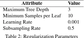
example, after 1800 iterations no real gain can be expected from adding more trees. To prevent such a behavior during the model building process, different regularization techniques are used. We introduced the four restricting parameters maximum tree depth, number of samples per leaf, learning rate and subsampling to lead the model building into the right direction. The maximum tree depth was binded to three, building a large number of trees with low depth is a general technique to avoid over-fitting. The influence of single and not representative outliers in the set of random samples should be minimized. This can be ensured by giving a minimum number of samples per leaf for the tree grow-ing process. We have decided to have at least ten samples per leaf, as we’re convinced that making a split leading to leafs with less then ten samples would lead to an unrepresentative response function. The learning rate, which can be considered as a weight-ing factor for each sweight-ingle tree, is 0.001. As the methodology of GBRT is to some degree comparable with the method of steepest descent, this factor can be considered as a factor lowering the step length whilst not influencing the step direction. The big number of 1800 trees in combination with the low learning rate ensures a quite moderate decrease in the model error leading towards the optimal combination of regularization parameters. By introduc-ing stochasticity into the model buildintroduc-ing process, variance and bias of the final model can also be minimized. Subsampling is a common technique to introduce stochasticy by just taking a ran-dom subsample of the training data sets per boosting iteration into account. We used just 50 percent of the available training data sets per boosting iteration. Table 2 gives an overview of the mentioned and used regularization parameters.
Attribute Value
Maximum Tree Depth 3
Minimum Samples per Leaf 10
Learning Rate 0.001
Subsampling Rate 0.5
Table 2: Regularization Parameters
The final model has a RMSE of 3.28 and a coefficient of determi-nation ofR2= 0.78.
5. CONCLUSIONS AND FUTURE WORK
A new approach for predicting wind speeds using GBRT is pre-sented. We see that GBRT in conjunction with established DEM based predictors are capable to model the complex behaviour of wind streams over a large mountainous area. The results are reli-able within a given accuracy.
(a) Relative Predictor Influence (b) Deviance over Boosting Steps
Figure 3: Model Description
the degree of dominance or enclosure of a location on an irregu-lar surface like a DEM (Yokoyama et al., 2002). Another quite promising approach would be to add indexes which make use of flow routing algorithms. Lindsay and Rothwell (Lindsay and Rothwell, 2008) introduced the Channelling and Deflection In-dex (CDI), a sophisticated algorithm which leaves the ray-tracing domain and makes also usage of multiple flow direction (MFD) algorithms to simulate the complex behaviour of air streams. Dif-ferent possible MFDs are named, probably the most promising for future investigations is D∞ (Tarboton, 1997).
Tuning the parameters of the GBRT is a iterative and subjective task. Finding the optimal parameter set and handling the trade-offs between number of trees, learning rate, tree depth and others needs to be carried out by an experienced operator. Grid search can be adopted to test a certain number of possible combinations of different parameters, pointing to an optimal set with respect to a given loss function. Techniques like global optimization do-main would probably lead to better results, for example evolu-tionary algorithms or genetic algorithms.
ACKNOWLEDGEMENTS
The author wants to thank the Federal Office of Meteorology and Climatology MeteoSwiss for the provision of the gust speed mea-surements. Furthermore the author wants to thank Prof. Anthony Lehmann from University of Geneva for correspondance and ad-vice.
REFERENCES
Antoni´c, O. and Legovi´c, T., 1999. Estimating the direction of an unknown air pollution source using a digital elevation model and a sample of deposition. Ecological Modelling 124(1), pp. 85–95.
Breiman, L., Friedman, J., Olshen, R. and Stone, C., 1984. Clas-sification and Regression Trees. Wadsworth and Brooks, Mon-terey, CA.
Cawsey, E., Austin, M. and Baker, B., 2002. Regional vegetation mapping in australia: a case study in the practical use of statistical modelling. Biodiversity & Conservation 11(12), pp. 2239–2274.
Chapman, L., 2000. Assessing topographic exposure. Meteoro-logical Applications 7, pp. 335–340.
de Rooy, W. C. and Kok, K., 2004. A Combined PhysicalSta-tistical Approach for the Downscaling of Model Wind Speed. Weather and Forecasting 19(3), pp. 485 – 495.
Elith, J., Leathwick, J. R. and Hastie, T., 2008. A working guide to boosted regression trees. Journal of Animal Ecology 77(4), pp. 802–813.
Farr, T., Rosen, P., Caro, E., Crippen, R., Riley, D., Hensley, S., Kobrick, M., Paller, M., Rodriguez, E., Roth, L., Seal, D., Shaf-fer, S., Shimada, J., Umland, J., Werenr, M., Oskin, M., Burbank, D. and Alsdorf, D., 2007. The shuttle radar topography mission. Reviews of Geophysics.
Garcia, M. and Boulanger, P., n.d. Low Altitude Wind Simula-tion over Mount Saint Helens Using NASA SRTM Digital Terrain Model.
Hastie, T., Tibshirani, R. and Friedman, J., 2001. The Elements of Statistical Learning. Springer Series in Statistics, Springer New York Inc., New York, NY, USA.
Heneka, P. and Ruck, B., 2004. Development of a storm dam-age risk map of germany - a review of storm damdam-age functions. In: Proceedings of the International Conference for Disasters and Society, Karlsruhe, 2004.
Hofherr, T. and Kunz, M., 2010. Extreme wind climatology of winter storms in Germany. Climate Research 41(2), pp. 105 – 123.
Leathwick, J., Rowe, D., Richardson, J., Elith, J. and Hastie, T., 2005. Using multivariate adaptive regression splines to predict the distributions of New Zealand’s freshwater diadromous fish. Freshwater Biology 50(12), pp. 2034–2052.
Lehmann, A., Leathwick, J. and Overton, J., 2002a. Assessing new zealand fern diversity from spatial predictions of species as-semblages. Biodiversity & Conservation 11(12), pp. 2217–2238.
Lehmann, A., Overton, J. M. and Leathwick, J. R., 2002b. GRASP: generalized regression analysis and spatial prediction. Ecological Modelling 160(12), pp. 165 – 183.
Lindsay, J. and Rothwell, J., 2008. Modelling channelling and deflection of wind by topography. In: Q. Zhou, B. Lees and G.-a. Tang (eds), Advances in Digital Terrain Analysis, Lecture Notes in Geoinformation and Cartography, Springer Berlin Heidelberg, pp. 383–406.
Overton, J., Theo Stephens, R., Leathwick, J. and Lehmann, A., 2002. Information pyramids for informed biodiversity conserva-tion. Biodiversity & Conservation 11(12), pp. 2093–2116.
Figure 4: max. Wind Speed map
Reiche, M., Funk, R., Zhang, Z., Hoffmann, C., Reiche, J., Wehrhan, M., Li, Y. and Sommer, M., 2012. Application of satellite remote sensing for mapping wind erosion risk and dust emission-deposition in inner mongolia grassland, china. Grass-land Science 58(1), pp. 8–19.
Riley, S. J., Degloria, S. D. and Elliot, R., 1999. A terrain rugged-ness index that quantifies topographic heterogeneity. Intermoun-tain Journal of Sciences 5(1-4), pp. 23–27.
Tarboton, D. G., 1997. A new method for the determination of flow directions and upslope areas in grid digital elevation models. Water Resources Research 33, pp. 309–319.
Weiss, A.-D., 2001. Topographic position and landforms anal-ysis. Poster Presentation, ESRI Users Conference, San Diego, CA.
Wilson, J. and Gallant, J., 2000. Terrain Analysis: Principles and Applications. Earth sciences: Geography, Wiley.
Winstral, A. and Marks, D., 2002. Simulating wind fields and snow redistribution using terrain-based parameters to model snow
accmulation and melt over a semi-arid mountain catchment. Hy-drologic Processes 16, pp. 3585–3603.
Yokoyama, R., Shlrasawa, M. and Pike, R. J., 2002. Visualizing topography by openness: a new application of image processing to digital elevation models: Photogrammetric engineering & re-mote sensing, v.