Agriculture, Ecosystems and Environment 82 (2000) 57–71
The role of climatic mapping in predicting the potential
geographical distribution of non-indigenous pests
under current and future climates
R.H.A. Baker
a,∗, C.E. Sansford
a, C.H. Jarvis
b,
R.J.C. Cannon
a, A. MacLeod
a, K.F.A. Walters
aaCentral Science Laboratory, Sand Hutton, York YO41 1LZ, UK
bDepartment of Geography, University of Edinburgh, Drummond Street, Edinburgh EH8 9XP, UK
Abstract
Climatic mapping, which predicts the potential distribution of organisms in new areas and under future climates based on their responses to climate in their home range, has recently been criticised for ignoring dispersal and interactions between species, such as competition, predation and parasitism. In order to determine whether these criticisms are justified, the different procedures employed in climatic mapping were reviewed, with examples taken from studies of the Mediterranean fruit fly (Ceratitis capitata), Karnal bunt of wheat (Tilletia indica) and the Colorado potato beetle (Leptinotarsa decemlineata). All these studies stressed the key role played by non-climatic factors in determining distribution but it was shown that these factors, e.g., the availability of food and synchrony with the host plant, together with the difficulties of downscaling and upscaling data, were different to those highlighted in the criticisms. The extent to which laboratory studies onDrosophila
populations, on which the criticisms are based, can be extrapolated to general predictions of species distributions was also explored. TheDrosophilaexperiments were found to illustrate the importance of climate but could not accurately determine potential species distributions because only adult and not breeding population densities were estimated. The experimental design overestimated species interactions and ignored other factors, such as the availability of food. It was concluded that while there are limitations, climatic mapping procedures continue to play a vital role in determining what G.E. Hutchinson defined as the “fundamental niche” in studies of potential distribution. This applies especially for pest species, where natural dispersal is generally less important than transport by man, and species interactions are limited by the impoverished species diversity in agroecosystems. Due to the lack of data, climatic mapping is often the only approach which can be adopted. Nevertheless, to ensure that non-climatic factors are not neglected in such studies, a standard framework should be employed. Such frameworks have already been developed for pest risk analyses and are suitable for general use in studies of potential distribution because, in order to justify the phytosanitary regulation of international trade, they must also consider the potential for pests to invade new areas and the impacts of such invasions. © 2000 Elsevier Science B.V. All rights reserved.
Keywords:Climatic mapping; Climate change; Pest risk analysis
∗Corresponding author. Tel.:+44-1904-462220; fax:+44-1904-462250.
E-mail address:[email protected] (R.H.A. Baker).
1. Introduction
Predicting the potential distribution of all pests (in this paper, “pests” include pathogens), both indige-nous and non-indigeindige-nous, plays a key role in deter-mining the effects of global change on agricultural, horticultural and forestry ecosystems. Inaccuracies in predicting potential distribution will impair our ability to identify the regions, commodities and ecosystems which are most vulnerable, to quantify crop losses and other impacts which may occur and to formulate ef-fective management strategies — all key objectives of Focus 3 of the Global Change and Terrestrial Ecosys-tems programme (Sutherst et al., 1996). These objec-tives also emulate the process of pest risk analysis (PRA) which is undertaken by plant protection organi-sations to determine the risks posed by non-indigenous pests and to justify any phytosanitary measures taken to combat the threat. Agreement on the techniques which are appropriate for predicting potential pest dis-tributions is therefore extremely important both for studies of global change and for plant quarantine. PRA also needs to take global change into account, be-cause, once established, the economic impact caused by non-indigenous pests, such as warmth loving in-sects or warm climate fungal pathogens, may increase. Climatic mapping, reviewed by Messenger (1959), Meats (1989) and Sutherst et al. (1995) for insects and by Coakley et al. (1999) for pathogens, is the princi-pal method for predicting potential distribution under current and future climates. However, it has recently been criticised by Davis et al. (1998a,b), who describe this technique for predicting species distributions as being “mistaken” and “invalidated” by species dis-persal and species interactions and by Lawton (1998) who considers that the null hypothesis — that distri-butions of organisms are solely determined by physi-ological tolerances — must be wrong and that it may never be possible to predict the future distribution and abundance of particular species even if reliable climate predictions are provided. Hodkinson (1999) has al-ready responded to these criticisms, stressing the role of ecophysiological models in predicting, e.g., the dis-tribution of herbivorous insects and soil arthropods at northern and altitude range limits and urging caution in making general inferences from narrowly limited laboratory experiments. In this paper, the justification for these criticisms is explored further. Examples of
the techniques used in climatic mapping are given and the extent to which theDrosophilaexperiments can be extrapolated to general predictions of species distribu-tions is explored. To ensure that future consideration is given to all relevant factors, a framework for predict-ing potential distribution, based on international PRA schemes is proposed.
2. Climatic mapping
The process of mapping a pest’s potential distribu-tion based on climate varies according to the amount of information available concerning its current distri-bution and its responses to climatic variables. Three levels of sophistication can be identified: comparisons of climate based on knowledge of a pest’s current distribution but where climatic factors relevant to the pest are unknown (Section 2.1), comparisons where relevant factors are known or have been inferred (Sec-tion 2.2) and models which predict environmental suitability based on phenology with or without con-sideration of responses to climatic extremes (Section 2.3). Examples of each are given to aid discussion.
2.1. Climatic comparisons based on pest distributions
At its simplest, the process of climatic mapping ex-amines the climate in an organism’s home range and compares it with the climate in the area being assessed for potential colonisation or the climate in the same areas under a climate change scenario. Graphs directly comparing seasonal variations in monthly means of climatic variables at weather stations, e.g., from the UK Meteorological Office (1972), or contained in the computer program, CLIMEX (Skarratt et al., 1995), may be drawn with 6-month displacements of calen-dar months to ensure that periods of climatic extremes, such as winters in northern and southern hemispheres, coincide.
R.H.A. Baker et al. / Agriculture, Ecosystems and Environment 82 (2000) 57–71 59
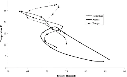
Fig. 1. Climograph for the Mediterranean fruit fly,C. capitata, based on mean monthly 1931–1960 climate data. Data for consecutive months from January to December are connected with a line.
the Mediterranean fruit fly, C. capitata, with mean monthly 1931–1960 temperature and relative humi-dity (RH) data from three weather stations extracted from CLIMEX (Fig. 1). Rotterdam is representative of several locations in northern Europe where popu-lations may breed in summer but die out in winter (Fischer-Colbrie and Busch-Petersen, 1989) due to low temperatures and absence of fruit which larvae require for survival (Papadopoulos et al., 1996). In Naples,C. capitatais only occasionally abundant and an important pest (Fimiani, 1989), while Tampa (FL) was predicted by Bodenheimer (1951) to provide optimum conditions.
Data from additional weather stations can be added to such graphs to give a valuable visual indication of climatic similarity. As more and more stations and cli-matic variables are added, a climate response surface or climate envelope is created showing the climatic conditions characterising a species’ home range. Vari-ous methods have been used to analyse the complex patterns which can be created when comparing the
climate surfaces or envelopes between areas of current and potential distribution, with and without climate change. For example, Jeffree and Jeffree (1996) plot-ted mean temperatures in the warmest months against those in the coldest months and correlated them with the distributions of mistletoe,Viscum album, and the Colorado potato beetle, L. decemlineata. Beerling et al. (1995) used a locally weighted regression to compare the distribution of Japanese knotweed, Fal-lopia japonica, in eastern Asia with that in Europe based on the mean temperature of the coldest month, the annual temperature sum greater than 5◦C and the
ratio of actual to potential evapotranspiration. The bio-climate prediction system, BIOCLIM, matches thresh-olds and limits for 12 temperature and precipitation variables and has been used to predict the distribution of many organisms, e.g., the Australian grasshopper,
et al., 1993) procedures. The “match climates” option in CLIMEX takes a simpler approach by calculating a “match index”, which summarises the similarities between selected climatic features (monthly mean minimum and maximum temperatures, rainfall and rainfall pattern) at weather stations within and out-side a species’ home range (Sutherst et al., 1995). Although this index can be weighted to emphasise a particular climatic variable, the combined index is only designed to identify climatic homologues, providing a measure of similarity for meteorological variables in different places without reference to par-ticular species. Despite the non-specific nature of this index, some authors (e.g., Boag et al., 1995) have used it to map potential distribution.
Methods that predict potential distributions solely on combinations of climatic variables in the areas of current distribution may prove accurate for cer-tain species in particular areas but greater precision is generally achieved by selecting climatic variables and their thresholds according to biological responses which have been determined by experiment. An al-ternative method is to infer these responses from an examination of the factors limiting their current distri-bution, as described later in this paper. Nevertheless, climatic comparisons are useful where little is known about an individual organism or an area. They can also be applied when the objective is principally to de-termine the overall relationship between the climatic conditions in the home range or the source of a traded commodity with that in the area under threat. Thus, Baker and Bailey (1979) divided up the world dia-grammatically into three zones based on their similari-ties with the climate in UK. Zone 1 comprised the cool temperate areas of the world from which pests could be expected to survive outdoors, at least in southern areas of the UK. Organisms from Zone 2, the warm temper-ate areas with continental climtemper-ates, might be expected to survive in a few localities and under glass whereas those from Zone 3 could only be expected to survive in protected cultivation. Bennett et al. (1998) used weightings of the CLIMEX “match index” to search for climatic homologues between Southern Australia and the Mediterranean in an attempt to target col-lections of cultivars to locations where they may be preadapted to Southern Australian climatic conditions for breeding programmes. Global climatic similari-ties have also been used to define the world’s biomes
(Whittaker, 1975; Prentice et al., 1992). While it is recognised that many other factors affect species dis-tributions, agreement cannot be reached on the num-ber of world biomes and the limits cannot readily be defined, the biome concept still constitutes one of the most successful macroecological theories (Lawton, 1999). At a larger scale, biogeographical zones may be defined in a similar manner. For example, Carey et al. (1995) classified Scotland into 10 zones, by com-bining six climatic variables interpolated to a 10 km2 grid using maximum and minimum altitudes, distance from the sea and the distribution of nine major taxo-nomic groups as guiding variables.
2.2. Mapping climatic indices relevant to the species concerned
The climatic factors that limit the geographical distribution of a species are commonly inferred by statistical analysis of the climatic data noted above. Alternatively, or in addition, data on critical thresh-olds may be obtained from direct field observations in an organism’s home range, in protected cultivation or in controlled laboratory experiments.
2.2.1. Karnal bunt
An example of mapping the potential distribution of a pest based on relevant climatic indices is pro-vided by studies of Karnal bunt, a serious disease of wheat caused by the fungus, T. indica. The disease has recently been found in parts of southern USA. Concerned that the disease could be introduced to other areas through grain shipments, a number of PRAs have been undertaken to determine the risks of introduction and economic impact in northern USA (G. Peterson, pers. commun.), Australia (Murray and Brennan, 1998) and Europe (Sansford, 1998). These authors applied the work of Jhorar et al. (1992), who found a high correlation between a humid thermal index (HTI), defined as the RH in mid-afternoon di-vided by the maximum daily temperature, calculated at the time of wheat ear emergence, and disease in-cidence over a 19-year period in the central plain of Punjab in India. An HTI between 2.2 and 3.3 was shown to be particularly favourable for the disease.
R.H.A. Baker et al. / Agriculture, Ecosystems and Environment 82 (2000) 57–71 61
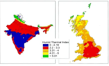
Fig. 2. Karnal bunt: mean HTIs for India in March 1961–1990.
Fig. 3. Karnal bunt: HTIs for Great Britain in June 1961–1990, with RHs corrected to represent values at 15:00 h.
which have been interpolated onto a grid according to geographical coordinates and elevation. World (New et al., 1999) and UK climatologies (Barrow et al., 1993), which interpolate 1961–1990 mean monthly data onto, respectively, a 0.5
◦ latitude ×
0.5
◦ longitude and a 10 km2grid, were used to map
HTIs for March in India (Fig. 2) and for June in UK (Fig. 3). Mean monthly RHs were calculated from vapour pressure using the formula provided by Gill (1982), divided by maximum temperatures to create mean daily HTIs and mapped with a GIS (ArcView, ESRI).
The critical HTI thresholds in Fig. 2 are in accord with the known distribution of the disease in India (Singh, 1994). However, the minimum value of daily HTI calculated from the 1961–1990 gridded climato-logy for UK in June was only 3.9, whereas Sansford (1998) found mean 1931–1960 HTIs for several UK weather stations to lie within the critical 2.2–3.3 range. Analysis of data from stations where RHs were recorded four times a day (at 3:00, 9:00, 15:00 and 21:00 h) revealed a significant difference between the
RHs at 15:00 h (as required by Jhorar et al., 1992, to estimate the mid-afternoon HTI) and the mean daily RH (the only parameter available from the global, European and UK climatologies). To determine the re-lationship between 15:00 h and daily mean RH in UK, RH and maximum temperature data were obtained from 39 English weather stations for June 1976 (Me-teorological Office, 1976) and HTIs were calculated from the daily mean RH and from the RH recorded at 15:00 h. Since the HTIs calculated from 15:00 h RH data were found to be, on average, 0.7±0.2 lower
than those obtained from mean daily RH data, a cor-rection factor of 0.7 was applied to UK HTIs. When mapped (Fig. 3), this showed that 230 10 km2 grid cells had HTIs within the critical 2.2–3.3 range, in an area covering much of central and southern England. June HTIs were also calculated and mapped from data derived from the second Hadley Centre coupled ocean–atmosphere global climate model (HadCM2) (Johns et al., 1997) and interpolated from 2.5
◦×3 .75
◦ latitude/longitude grid cells to a
0.5
◦ latitude×0 .5
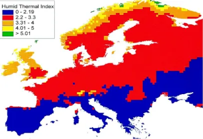
et al., 1995; Barrow, pers. commun.) (Fig. 4). The mean of four HadCM2 experiments with a high (1%) annual greenhouse gas forcing was used. The four experiments varied only in their initial start date. The scenario predicts climate change at 2050, representing a mean for the 30-year period, 2035–2064, with global mean CO2 concentrations reaching 515 ppmV.
Com-pared to the 1961–1990 period, global warming for this scenario is predicted to reach a mean of 1.91◦C
(range 1.88–1.97), with Europe warming on average by 2.30◦C (range 2.09–2.57) (Johns et al., 1997).
Fig. 4 shows that large areas of the UK and Europe are predicted to have daily June HTIs in the critical range for Karnal bunt by 2050. However, this repre-sents only one part of the investigation. Mean daily HTIs are used and a conversion to mid-afternoon HTIs is required. The specific phenological stage of wheat at whichT. indicacan infect and cause disease is still incompletely specified, however, the stage is likely to be between boot and anthesis. The HTIs are only significant at this stage and its timing will need to be predicted throughout Europe for the main bread and durum wheat cultivars before a map defining Karnal bunt risk can be produced. Since wheat ear emergence may only occur over a short period (app-roximately 14 days in southern England under cur-rent conditions) and does not coincide with calendar months, ongoing research is investigating the genera-tion of daily data from monthly data applied to bread and durum wheat phenology models (Porter, 1993; Miglietta, 1991) to determine the critical periods for infection under current and future climates. This study forms part of a wider Project entitled “Karnal bunt risks” (QLK5CT-1999-01554) which is financed by the European Commission under the Quality of Life and Management of Living Resources Programme; one of the four thematic programmes of the EC Fifth Framework R & D Programme. The Project does not necessarily reflect the views of the Commission and in no way anticipates the Commission’s future policy in this area.
Mapping relevant climatic indices to predict dis-tribution has been particularly successful with plants (Woodward, 1987). For example, Cathey (1990) divided North America into 11 zones and nine sub-zones based on annual minimum temperatures, as-signing particular plant species to zones and subzones based on knowledge of their winter hardiness. Maps
of potential distribution for current and future cli-mates have also been created for crop cultivars, e.g., for grapes (Kenny and Shao, 1992) and have bene-fited from the availability of interpolated climates (e.g., Booth and Jones, 1998).
2.3. Predicting development and survival
Many plant and pest distributions can only rarely be directly related to one over-riding climatic vari-able, such as risk of frost. In most cases, a variety of interrelated factors may be significant in determining whether conditions are suitable for both development and survival. Sutherst et al. (1995) have criticised the deductive approach, where predictions of geographi-cal distribution are based solely on the accumulation of experimental data, which may be difficult to relate to field conditions, and even after long and very de-tailed investigations (e.g., Morris and Fulton, 1970), can never uncover all key factors. However, Rogers (1979) showed, in studies of tsetse flies, that where extensive field population records are available and mortalities can be estimated and incorporated into climographs, distributions can be inferred from field data. The collection of some data, such as the number of degree-days above a critical threshold temperature needed to complete particular life stages and the day lengths and temperature combinations triggering di-apause, has almost universal applicability, since they can be used in phenology models (see Section 2.3.1) which predict the rate of development.
Predicting the climatic factors that determine sur-vival, such as overwinter, is significantly more chal-lenging (Leather et al., 1993). Much of the available published literature is limited to exposing populations outdoors under containment, e.g., in cages to observe overwintering survival. This limits effective interpre-tation (Macdonald and Walters, 1996). Baker (1972) proposed that examining the climatic responses of na-tive species in areas threatened by colonisation may reveal the key factors in common required for sur-vival. Bale and Walters (pers. commun.) have used this approach to predict cold hardiness in UK. Over-wintering survival under field conditions for the eight insect species studied was found to be correlated with laboratory estimates of the time for 50% mortality at
−5◦C. A combination of such direct observations of
R.H.A. Baker et al. / Agriculture, Ecosystems and Environment 82 (2000) 57–71 63
Fig. 4. Karnal bunt: HTIs for Europe in June 2050 under the HadCM2 global climate model.
of climatic conditions in an organism’s current distri-bution, as employed by CLIMEX (see Section 2.3.2), offers the most reliable solution available from current knowledge.
2.3.1. Phenology models
Phenology models are designed to predict the tim-ing of events durtim-ing an organism’s life cycle in a particular area based on knowledge of the critical climatic thresholds. These are based on the physiolog-ical findings of authors such as Sharpe and deMichele (1977) who found a close relationship between insect development and temperature. They can also be used to predict potential distribution if organisms have to reach a particular stage in their life cycle in order to survive a period of climatic stress, such as winter, and the timing of such a stage can be predicted. They are dependent on complete daily sets of weather data, such as sequential daily maximum and minimum temperatures, but these data are collected at point sources, weather stations, which may be at a con-siderable distance and in very different terrain from those areas where crops are grown. In order to map phenologies over the landscape, the model outputs, usually the Julian dates at which a pest is expected to reach a particular stage, may be interpolated using one of a variety of algorithms, e.g., trend surface analysis (e.g., Schaub et al., 1995). A second, more unusual, strategy is to model phenology according to the na-ture of continuous spatially derived inputs at discrete (gridded) intervals over the landscape (Jarvis, 1999). While this second methodology is more computation-ally intensive, the results have been shown to preserve more closely the underlying spatial autocorrelation of the phenologies and to maintain a logical biolo-gical sequence between pest stages that may be lost when interpolating point phenologies (Jarvis et al., 1999). An example of this latter approach is provided here.
In computing Fig. 5, daily maximum and minimum temperatures were interpolated throughout England and Wales for the period 1 January–31 October for years with unusually hot (1976) and cool (1986) sum-mers. The temporal sequence of results for each 1 km2 grid of the landscape, together with geographically de-termined estimates of photoperiod, were used to run a linear multi-stage phenology model for Colorado bee-tle (Baker and Cohen, 1985) at each discrete location.
Given the likelihood that small errors when estimating daily temperatures might propagate rapidly through-out a run of the phenology model, a more sophisticated interpolation model, partial thin plate splines, (Hutchinson, 1991) was used when interpolating tem-peratures rather than the cruder trend surface methods of previous work constructing spatial phenologies. The interpolation method also incorporated factors such as elevation, distance from the sea, cold air drainage and urban heating through the use of gridded digital data manipulated within a proprietary GIS.
The model run illustrated in Fig. 5 has been cur-tailed on 31 October, beyond which point it is as-sumed that there will be insufficient food for the emerging adults to feed on in preparation for dia-pause. When running the phenology model in this example, the starting conditions assumed that a viable nominal population of overwintered Colorado beetle immature adults were present throughout the land-scape. In this sense, the geographical results represent a “worst case” scenario of the problems the pest might present in England and Wales should it become established, with the area at risk varying between ap-proximately 120,000 km2 in 1976 (an exceptionally hot summer) to 46,000 km2in 1986 (a cool summer). Investigating the extent of insect development in ex-treme years allows the assessment of the probable bounds over which an insect might survive; this is preferable to reliance on a single “average” extent inherent in the use of climate normal (30-year aver-aged) data which has the potential to underestimate extreme risk. Sequences of years can also be studied to help predict the potential for long-term establish-ment. The use of daily data, rather than monthly data, has additional advantages. Most insects have a short development cycle, so daily predictions are more ap-propriate, especially when it is necessary to combine insect and crop models to predict development and survival.
2.3.2. CLIMEX
distri-R.H.A. Baker et al. / Agriculture, Ecosystems and Environment 82 (2000) 57–71 65
bution and any experimental information for growth and stress, such as degree-days for development and critical photoperiods, are combined to produce an ecoclimatic index (EI), a measure of the suitability of a location for establishment.
Originally based on weather station data, climato-logical data interpolated into grid cells have increas-ingly been used (e.g., Baker et al., 1996; Yonow and Sutherst, 1998), to reflect more accurately the rela-tionship between climate and landscape. Grids created by downscaling global climate models can also be used to explore changes in the EI under global change. Baker et al. (1998) adopted this approach to study the effect of climate change on the potential distribution
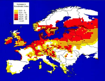
Fig. 6. The increase in the EI for Colorado beetle predicted by CLIMEX under the mean HadCM2 greenhouse gas climate change scenario in Europe. The EI estimates the suitability of the location for establishment.
of Colorado Beetle in Europe. As for Karnal bunt, the mean of four HadCM2 experiments with a high (1%) annual greenhouse gas forcing was input to CLIMEX and EIs were calculated and mapped with a GIS. For Great Britain, we found that this global change scenario would provide 79 additional 0.5
◦ latitude×
0.5
◦ longitude grid cells climatically suitable for
colonisation by Colorado beetle, representing a po-tential range expansion of 120% and a mean northerly increase of 3.5◦latitude (400 km). This expected
3. Critique of climatic mapping
3.1. Experiments with Drosophila populations
Davis et al. (1998a,b) studied the population dy-namics of threeDrosophilaand one insect parasitoid species in temperature clines created by connecting four incubators set at constant temperatures of 10, 15, 20 and 25◦C with tubes which allowed the adults to
move along the cline. Global warming was mimicked by increasing temperatures by 5◦C in each incubator.
Weekly adult population levels were counted and the means for weeks 5–25 compared. They found signi-ficant differences in the distribution of adults of all the Drosophilaspecies along the clines according to whether each species was able to develop in isolation or in competition with others and whether they were subjected to attack by the insect parasitoid. While species distributions were influenced by temperature, they could not have been predicted by temperature alone, and dispersal and species interactions were critical to determining abundance along the cline. It was concluded that potential geographical distribu-tions cannot be accurately predicted without taking dispersal and species interactions, such as competition and the effect of natural enemies, into account and that, therefore, attempts to predict the potential distri-butions of organisms solely using climatic mapping are mistaken and invalid.
3.2. Discussion
Following such a study, two key questions must be addressed: to what extent can the results from their experimental system be extrapolated to studies of potential geographical distribution under current and future climates and do climatic mapping stud-ies ignore the importance of dispersal and specstud-ies interactions?
3.2.1. Extrapolating studies of Drosophila populations to general predictions of species distributions
The primary objective in studies of the potential distribution of pests, whether or not climatic mapping methods are used, is to determine whether the estab-lishment of any breeding colonies is possible. Once the potential for establishment has been determined,
additional work is then undertaken to try and pre-dict whether population levels will exceed economic thresholds and to estimate the rate of dispersal within the crops at risk. A similar sequence of study is also logical when estimating the potential distribution of crops and wild organisms. This well-established pro-cess of investigation follows Hutchinson (1957), who distinguished the fundamental niche, based on physi-cal factors in the environment, from the realised niche, which depends on biotic factors.
Davis et al. (1998a,b) found that, without interspe-cific competition and when dispersal was prevented,
D. subobscura became extinct at 25◦C and both D. melanogasterandD. simulansdied out at 10◦C. This is clear evidence of the fundamental role of tempera-ture in determining distribution, since, although some breeding may occur for a short period, we can con-clude that establishment is still not possible irrespec-tive of the method or rate of dispersal of adults into chambers at these temperatures and the role of species interactions in influencing such movement. In the rest of the cline, where temperatures are suitable for all species to establish, dispersal and species interac-tions may indeed play significant roles in influencing population breeding.
It is, of course, possible that, in areas where phy-sical factors are not limiting, poor dispersal and in-teractions with competitors and natural enemies may lead to the extinction of all individuals and breed-ing colonies. However, before such factors within the realised niche are considered, it is of greater impor-tance to determine whether there is sufficient food for survival. Although theDrosophila experiments were not designed to study this, in most cases, the avail-ability of food, e.g., host plants for pests, will be of much greater importance than dispersal and species interactions.
The distribution along the clines in theDrosophila
R.H.A. Baker et al. / Agriculture, Ecosystems and Environment 82 (2000) 57–71 67
result, where dispersal along the cline was allowed, adults dispersing from other chambers could not be distinguished from those reared in each chamber and thus the degree to which the observed distributions were due to breeding success in the different cham-bers or adult movement alone cannot be determined and the role of dispersal in establishing populations may have been overestimated.
Nevertheless, natural dispersal clearly plays a sig-nificant role in determining potential distributions and population densities after establishment. However, for many pest species, apart from those which do migrate long distances, transport by humans to new areas is generally more important than natural dispersal. The role of humans in dispersing organisms throughout the world has been well documented and research on the implications of such species invasions and the degree to which the results can be predicted is in-tensifying (Williamson, 1996, 1999). The problem is greatest for crop pests. In some countries, such as the USA, 40% are of alien origin, having been introduced by man (Pimentel, 1984). While most countries have enacted strong legislation to prevent the deliberate release of alien organisms, the continuing increase in the frequency, speed and volume of trade in plant commodities is maintaining a high risk of pest entry. For example, in 1995, the UK Central Science Lab-oratory received over 5000 samples of invertebrates intercepted on plants and plant products imported into England and Wales. Approximately 560 taxa were identified, belonging to 169 families. This represents only a small proportion of insects being carried into England and Wales since not all imported material is examined. As such, and especially for crop pests, nat-ural dispersal may play only a minor role in spreading populations to new areas.
Although no direct estimates of mortality from interspecific competition and parasitism have been published from the Drosophila experiments, they are likely to have been very much higher than those expected in natural environments because the exper-imental set up allowed only minimum temporal and spatial niche differentiation and dispersal. In the natu-ral world, competition betweenDrosophilaspecies is greatly reduced by the exploitation of different foods, with a significant temporal separation in periods of greatest abundance (Shorrocks, 1975; Baker, 1979). Parasitization rates, can also vary considerably
dur-ing the year and between different substrates, with many parasitoids discriminating between different
Drosophila hosts and their food substrates (Baker, 1979; Janssen et al., 1998; Eijs, 1999).
When organisms are introduced to new areas, pop-ulation explosions are frequently observed because of the absence of natural enemies, e.g., Ohgushi and Sawada (1998). Such events happen more frequently in man-made environments such as agricultural crops which have an impoverished diversity of fauna and flora. Biological control agents may need to be col-lected from the organism’s home range and released to provide satisfactory control. Species interactions may prevent establishment (Lawton and Brown, 1986) but their impact is likely to be greater in natural environ-ments or where biological control agents are being in-troduced into an agroecosystem when natural enemies and competitors are already present. For pathogens, such species interactions are likely to be far less im-portant in determining whether colonisation of a new area is successful; other factors such as the extent of host resistance will generally be far more significant.
3.2.2. Do climatic mapping studies ignore other factors?
the biotic and abiotic factors have been assessed, establishment can still only be predicted by taking into account other factors intrinsic to each species. Both genetic variability (Kennedy, 1993), which de-termines a species adaptability to the natural and artificial environment, and the reproductive strategy, which defines the extent to which populations can be sustained at low levels, also need to be considered.
Even if data for all these factors are available, con-siderable additional interpretation of the data may be required. For example, climatic data may still need spatial and temporal downscaling to model a particu-lar situation with sufficient accuracy or upscaling to enable broad predictions to be made. Long-term, e.g., 30 years, data may not show the effect of certain co-incidences, such as a sequence of cool, short summers or growth seasons. Climatic variation in a pest’s home range may not be comparable to that in the area at risk. Climate responses cannot be readily averaged for all stages in the life cycle and establishment may depend on very short-term weather events, e.g., for mating and egg laying (Baker, 1972).
4. Conclusions
This survey of climatic mapping techniques and the critical examination of the Drosophila experiments by Davis et al. (1998a,b) have both confirmed that climatic mapping has a central role to play in predict-ing the potential distribution of organisms under cur-rent and future climates and supported Hodkinson’s (1999) view that their conclusions neglect the fact that many species distributions can be predicted ac-curately by good ecophysiological studies linked to relevant climatic data. Despite potential limitations resulting from habitat-related differences between ac-tual and projected distributions, climatic mapping is useful in determining the maximum limits of estab-lishment based on Hutchinson’s (1957) concept of the fundamental niche. It may be particularly relevant to studies of man-made agricultural environments, since pests are frequently transported by man and interactions with competitors and natural enemies are generally limited by crop management techniques and the structure of the agroecosystem. It is also recognised that other habitat factors, such as host distribution and existing pest management practices,
acting individually or in combination, will generally play important roles (Pimentel, 1993).
Difficulties, such as downscaling and upscaling is-sues, arise in the interpretation and use of current and global change climate data. In addition, the iden-tification and modelling of an organism’s responses to climate, whether based on deductive or inductive methods, will contain errors. Nevertheless, in many cases, climatic mapping provides the only method that can be used due to insufficient data on other factors. Host distribution may be readily available and its role in defining potential distribution rapidly assessed, but even where data on species interactions and dispersal are well known, interpretation and prediction are ex-tremely difficult (Lawton, 1999; Williamson, 1999). Pragmatically, therefore, when decisions on poten-tial distributions must be made, e.g., in plant quaran-tine, and release in quarantine containment is not an option or would not provide relevant data, climatic mapping techniques often provide the only method available.
R.H.A. Baker et al. / Agriculture, Ecosystems and Environment 82 (2000) 57–71 69
established, new pests may increase their economic impact as the climate changes.
Acknowledgements
We gratefully acknowledge the assistance of Elaine Barrow and Mike Hulme of the Climatic Research Unit, University of East Anglia for the provision of climatic datasets and Plant Health Division of MAFF for funding this paper.
References
Baker, C.R.B., 1972. An approach to determining potential pest distribution. EPPO Bull. 3, 5–22.
Baker, R.H.A., 1979. Studies on the interactions between
Drosophilaparasites. Doctorate Thesis. University of Oxford, Oxford.
Baker, C.R.B., Bailey, A.G., 1979. Assessing the threat to British crops from alien diseases and pests. In: Ebbels, D.L., King, J.E. (Eds.), Plant Health. Blackwell Scientific Publications, Oxford, pp. 43–54.
Baker, C.R.B., Cohen, L.I., 1985. Further development of a computer model for simulating pest life cycles. EPPO Bull. 15, 317–324.
Baker, R.H.A., Cannon, R.J.C., Walters, K.F.A., 1996. An asse-ssment of the risks posed by selected non-indigenous pests to UK crops under climate change. Aspects Appl. Biol. 45, 323– 330.
Baker, R.H.A., MacLeod, A., Cannon, R.J.C., Jarvis, C.H., Walters, K.F.A., Barrow, E.M., Hulme, M., 1998. Predicting the impacts of a non-indigenous pest on the UK potato crop under global climate change: reviewing the evidence for the Colorado beetle,
Leptinotarsa decemlineata. In: Proceedings of the Brighton Crop Protection Conference on Pests and Diseases, Vol. III, pp. 979–984.
Barrow, E.M., Hulme, M., Jiang, T., 1993. A 1961–90 baseline climatology and future climate change scenarios for Great Britain and Europe. Part I: 1961–90 Great Britain baseline climatology. Climatic Research Unit, Norwich, 43 pp. (plus maps).
Beerling, D.J., Huntley, B., Bailey, J.P., 1995. Climate and the distribution ofFallopia japonica: use of an introduced species to test the predictive capacity of response surfaces. J. Veg. Sci. 6, 269–282.
Bennett, S.J., Saidi, N., Enneking, D., 1998. Modelling climatic similarities in Mediterranean areas: a potential tool for plant genetic resources and breeding programmes. Agric. Ecosyst. Environ. 70, 129–143.
Boag, B., Evans, K.A., Yeates, G.W., Johns, P.M., Neilson, R., 1995. Assessment of the global potential distribution of the predatory land planarianArtioposthia triangulata(Dendy) (Tricladida: Tericola) from ecoclimatic data. NZ J. Zool. 22, 311–318.
Bodenheimer, F.S., 1951. Citrus Entomology in the Middle East. Junk, Gravenhage.
Booth, T.H., Jones, P.G., 1998. Identifying climatically suitable areas for growing particular trees in Latin America. For. Ecol. Mgmt. 108, 167–173.
Carey, P.D., Preston, C.D., Hill, M.O., Usher, M.B., Wright, S.M., 1995. An environmentally defined biogeographical zonation of Scotland designed to reflect species distributions. J. Ecol. 83, 833–845.
Carpenter, G., Gillison, A.N., Winter, J., 1993. DOMAIN: a flexible modelling procedure for mapping potential distributions of plants and animals. Biodivers. Conserv. 2, 667–680. Cathey, H.M., 1990. USDA plant hardiness zone map. USDA
Agric. Res. Serv. Misc. Publ. 1475.
Coakley, S.M., Scherm, H., Chakraborty, S., 1999. Climate change and plant disease management. Annu. Rev. Phytopathol. 37, 399–426.
Cook, W.C., 1925. The distribution of the alfalfa weevil (Phytonomus posticusGyll.). A study in physical ecology. J. Agric. Res. 30, 479–491.
Davis, A.J., Lawton, J.H., Shorrocks, B., Jenkinson, L.S., 1998a. Individualistic species responses invalidate simple physiological models of community dynamics under global environmental change. J. Anim. Ecol. 67, 600–612.
Davis, A.J., Jenkinson, L.S., Lawton, J.H., Shorrocks, B., Wood, S., 1998b. Making mistakes when predicting shifts in species range in response to global warming. Nature (London) 391, 783–786.
Eijs, I.E.M., 1999. The evolution of resource utilisation in
Leptopilina species. Doctorate Thesis. University of Leiden, Leiden.
EPPO, 1997. Pest risk assessment scheme. EPPO Bull. 27, 281–305.
Fimiani, P., 1989. Mediterranean region. In: Robinson, A.S., Hooper, G. (Eds.), Fruit Flies: their Biology, Natural Enemies and Control, Vol. 3A. Elsevier, Amsterdam, pp. 39–50. Fischer-Colbrie, P., Busch-Petersen, E., 1989. Temperate Europe
and West Asia. In: Robinson, A.S., Hooper, G. (Eds.), Fruit Flies: their Biology, Natural Enemies and Control, Vol. 3A. Elsevier, Amsterdam, pp. 91–99.
Gill, A.E., 1982. Atmosphere and Ocean Dynamics. Academic Press, New York.
Hawksworth, D.L., Kirk, P.M., Sutton, B.C., Pegler, D.N., 1995. Ainsworth and Bisby’s Dictionary of the Fungi, 8th Edition. Commonwealth Mycological Institute, London.
Hodkinson, I.D., 1999. Species response to global environmental change or why ecophysiological models are important: a reply to Davis et al. J. Anim. Ecol. 68, 1259–1262.
Hulme, M., Conway, D., Jones, P.D., Jiang, T., Barrow, E.M., Turney, C., 1995. Construction of a 1961–90 European climatology for climate modelling and impacts applications. Int. J. Clim. 13, 1333–1363.
Hutchinson, G.E., 1957. Concluding remarks. Cold Spring Harbour Symp. Quant. Biol. 22, 415–427.
Janssen, A., Driessen, G., de Haan, M., Roodbol, N., 1998. The impact of parasitoids on natural populations of temperate woodlandDrosophila. Neth. J. Zool. 38, 61–73.
Jarvis, C.H., 1999. Insect phenology: a geographical perspective. Doctorate Thesis. University of Edinburgh, Edinburgh, UK. Jarvis, C.H., Stuart, N., Morgan, D., Baker, R.H.A., 1999.
To interpolate and thence to model, or vice versa? In: Gittings, B. (Ed.), Integrating Information Infrastructures with Geographical Information Technology. Taylor & Francis, London, pp. 229–242.
Jeffree, C.E., Jeffree, E.P., 1996. Redistribution of the potential geographical ranges of mistletoe and Colorado beetle in Europe in response to the temperature component of climate change. Funct. Ecol. 10, 562–577.
Jhorar, O.P., Mavi, H.S., Sharma, I., Mahi, G.S., Mathauda, S.S., Singh, G., 1992. A biometeorological model for forecasting Karnal bunt disease of wheat. Plant Dis. Rep. 7, 204–209. Johns, T.C., Carnell, R.E., Crossley, J.F., Gregory, J.M., Mitchell,
J.F.B., Senior, C.A., Tett, S.F.B., Wood, R.A., 1997. The second Hadley Centre coupled ocean–atmosphere GCM: model description, spinup and validation. Clim. Dyn. 13, 103–134. Kennedy, G.S., 1993. Impact of intraspecific variation on insect
pest management. In: Kim, K.C., McPheron, B.A. (Eds.), Evolution of Insect Pests. Wiley, New York, pp. 425–451. Kenny, G.J., Shao, J., 1992. An assessment of a
latitude–temperature index for predicting climate suitability for grapes in Europe. J. Hort. Sci. 67, 239–246.
Kohlmann, B., Nix, H., Shaw, D.D., 1988. Environmental predictions and distributional limits of chromosomal taxa in the Australian grasshopperCaledia captiva(F.). Oecologia 75, 483–493.
Lawton, J.H., 1998. Small earthquakes in Chile and climate change. Oikos 82, 209–211.
Lawton, J.H., 1999. Are there general laws in ecology. Oikos 84, 177–192.
Lawton, J.H., Brown, K.C., 1986. The population and community ecology of invading insects. Phil. Trans. R. Soc. London B 314, 607–617.
Leather, S.R., Walters, K.F.A., Bale, J.S., 1993. The Ecology of Insect Overwintering. Cambridge University Press, Cambridge. Macdonald, O.C., Walters, K.F.A., 1996. Overwintering potential ofLiriomyza huidobrensispupae in the UK. In: Walters, K.F.A., Kidd, N.A.C. (Eds.), Populations and Patterns in Biology. IPPP, Ascot, pp. 101–106.
Meats, A., 1989. Bioclimatic potential. In: Robinson, A.S., Hooper, G. (Eds.), Fruit Flies: their Biology, Natural Enemies and Control, Vol. 3B. Elsevier, Amsterdam, pp. 241–252. Messenger, P.S., 1959. Bioclimatic studies with insects. Annu.
Rev. Entomol. 4, 183–206.
Meteorological Office, 1972. Tables of Temperature, Relative Humidity, Precipitation and Sunshine for the World. Part III. Europe and the Azores. HMSO (Books), London.
Meteorological Office, 1976. Mon. Weath. Rep. 93 (6) 101–120. Miglietta, F., 1991. Simulation of wheat ontogenesis. II. Predicting
dates of ear emergence. Clim. Res. 1, 151–160.
Morris, R.F., Fulton, W.C., 1970. Models for the development and survival of Hyphantria cuneain relation to temperature and humidity. Mem. Entomol. Soc. Can. 70, 1–60.
Murray, G.M., Brennan, J.P., 1998. The risk to Australia from
Tilletia indica, the cause of Karnal bunt of wheat. Aust. Plant Pathol. 27, 212–225.
New, M., Hulme, M., Jones, P.D., 1999. Representing twentieth century space–time climate variability. Part 1: development of a 1961–90 mean monthly terrestrial climatology. J. Clim. 12, 829–856.
Ohgushi, T., Sawada, H., 1998. What changed the demography of an introduced population of a herbivorous lady beetle. J. Anim. Ecol. 67, 679–688.
Papadopoulos, N.T., Carey, J.R., Katsoyannos, B.I., Kouloussis, N.A., 1996. Overwintering of the Mediterranean fruit fly (Diptera: Tephritidae) in Northern Greece. Ann. Entomol. Soc. Am. 89, 526–534.
Pimentel, D., 1984. Biological invasions of plants and animals in agriculture and forestry. In: Mooney, H.A., Drake, J.A. (Eds.), Ecology of Biological Invasions of North America and Hawaii. Springer, London, pp. 149–162.
Pimentel, D., 1993. Habitat factors in new pest invasions. In: Kim, K.C., McPheron, B.A. (Eds.), Evolution of Insect Pests. Wiley, New York, pp. 165–181.
Porter, J.R., 1993. AFRCWHEAT2: a model of the growth and development of wheat incorporating responses to water and nitrogen. Eur. J. Agron. 2, 69–82.
Prentice, I.C., Cramer, W., Harison, S.P., Leemans, R., Monserud, R.A., Solomon, A.M., 1992. A global biome model based on plant physiology and dominance, soil properties and climate. J. Biogeogr. 19, 117–134.
Rogers, D., 1979. Tsetse population dynamics and distribution: a new analytical approach. J. Anim. Ecol. 48, 825–849. Sansford, C.E., 1998. Karnal bunt (Tilletia indica): detection of
Tilletia indicaMitra in the US: potential risk to the UK and the EU. In: Malik, V.S., Mathre, D.E. (Eds.), Bunts and Smuts of Wheat: An International Symposium, North Carolina, August 17–20, 1997. NAPPO, Ottawa, pp. 273–302.
Schaub, L.P., Ravlin, F.W., Gray, D.R., Logan, J.A., 1995. Landscape framework to predict phenological events for gypsy moth (Lepidoptera: Lymantriidae) management problems. Environ. Entomol. 24, 10–18.
Sharpe, P.J.H., deMichele, D.W., 1977. Reaction kinetics of poikilotherm development. J. Theor. Biol. 64, 649–670. Shorrocks, B., 1975. The distribution and abundance of woodland
species ofDrosophila(Diptera: Drosophilidae). J. Anim. Ecol. 44, 851–864.
Singh, A., 1994. Distribution and economic importance of Karnal bunt in Uttar Pradesh. In: Epidemiology and Management of Karnal Bunt Disease in Wheat. Research Bulletin No. 127. G.B. Pant University of Agriculture and Technology, p. 21. Skarratt, D.B., Sutherst, R.W., Maywald, G.F., 1995. CLIMEX for
Windows 1.0. Users Guide. CSIRO and CRC for Tropical Pest Management, St Lucia, Australia.
Sutherst, R.W., 1999. Climate change and invasive species — a conceptual framework. In: Mooney, H.A., Hobbs, R.J. (Eds.), Invasive Species in a Changing World. Island Press. Sutherst, R.W., Maywald, J.F., 1985. A computerised system for
R.H.A. Baker et al. / Agriculture, Ecosystems and Environment 82 (2000) 57–71 71
Sutherst, R.W., Maywald, G.F., Skarratt, D.B., 1995. Predicting insect distributions in a changed climate. In: Harrington, R., Stork, N.E. (Eds.), Insects in a Changing Environment. Academic Press, London, pp. 59–91.
Sutherst, R.W., Ingram, J.S.I., Steffen, W.I., 1996. GCTE activity 3.2 global change impacts on pests, diseases and weeds implementation plan. Global Change and Terrestrial Ecosystems Report No. 11. GCTE Core Project Office, Canberra. Walker, P.A., Cocks, K.D., 1991. HABITAT: a procedure for
modelling a disjoint environmental envelope for a plant and animal species. Global Ecol. Biogeogr. Lett. 1, 108–118.
Whittaker, R.H., 1975. Communities and Ecosystems, 2nd Edition. Macmillan, New York.
Williamson, M., 1996. Biological Invasions. Chapman & Hall, London.
Williamson, M., 1999. Invasions. Ecography 22, 5–12.
Woodward, F.I., 1987. Climate and Plant Distribution. Cambridge University Press, Cambridge.