Discussion Papers | OGC

(1)

Open Geospatial Consortium Inc.

Date: 2004-09-30

Reference number of this OGC™ project document: OGC 04-071

Version:1.0.0

Category: OGC™ Discussion Paper

Editor: Arliss Whiteside

Some image geometry models

Copyright notice

This OGC document is copyright-protected by OGC. While the reproduction of drafts in any form for use by participants in the OGC standards development process is permitted without prior permission from OGC, neither this document nor any extract from it may be reproduced, stored or transmitted in any form for any other purpose without prior written permission from OGC.

Warning

This document is not an OGC Standard. It is distributed for review and comment. It is subject to change without notice and may not be referred to as an OGC Standard.

Recipients of this document are invited to submit, with their comments, notification of any relevant patent rights of which they are aware and to provide supporting documentation.

Document type: OGC™ Discussion Paper Document stage: Final

(2)

NOTICE

Permission to use, copy, and distribute this document in any medium for any purpose and without fee or royalty is hereby granted, provided that you include the above list of copyright holders and the entire text of this NOTICE.

We request that authorship attribution be provided in any software, documents, or other items or products that you create pursuant to the implementation of the contents of this document, or any portion thereof.

No right to create modifications or derivatives of OGC documents is granted pursuant to this license. However, if additional requirements (as documented in the Copyright FAQ at http://www.opengeospatial.org/about/?page=ipr&view=ipr_faq) are satisfied, the right to create modifications or derivatives is sometimes granted by the OGC to individuals complying with those requirements. THIS DOCUMENT IS PROVIDED "AS IS," AND COPYRIGHT HOLDERS MAKE NO REPRESENTATIONS OR

WARRANTIES, EXPRESS OR IMPLIED, INCLUDING, BUT NOT LIMITED TO, WARRANTIES OF MERCHANTABILITY, FITNESS FOR A PARTICULAR PURPOSE, NON-INFRINGEMENT, OR TITLE; THAT THE CONTENTS OF THE

DOCUMENT ARE SUITABLE FOR ANY PURPOSE; NOR THAT THE IMPLEMENTATION OF SUCH CONTENTS WILL NOT INFRINGE ANY THIRD PARTY PATENTS, COPYRIGHTS, TRADEMARKS OR OTHER RIGHTS.

COPYRIGHT HOLDERS WILL NOT BE LIABLE FOR ANY DIRECT, INDIRECT, SPECIAL OR CONSEQUENTIAL DAMAGES ARISING OUT OF ANY USE OF THE DOCUMENT OR THE PERFORMANCE OR IMPLEMENTATION OF THE CONTENTS THEREOF.

The name and trademarks of copyright holders may NOT be used in advertising or publicity pertaining to this document or its contents without specific, written prior permission. Title to copyright in this document will at all times remain with copyright holders. RESTRICTED RIGHTS LEGEND. Use, duplication, or disclosure by government is subject to restrictions as set forth in subdivision (c)(1)(ii) of the Right in Technical Data and Computer Software Clause at DFARS 252.227.7013

OpenGIS®, OGC™, OpenGeospatial™ and OpenLS ® are trademarks or registered trademarks of Open Geospatial Consortium, Inc. in the United States and in other countries.

(3)

OGC 04-071

Figures

Page Figure 1 — A region of local linearity ... 8

(4)

i. Preface

This discussion paper contains the material that is still relevant from Section 6 (or Appendix A) of the previous version 4 (document OGC 99-107) of OGC Abstract Specification Topic 7, titled “The Earth Imagery Case”. That version of Topic 7 has now been superseded by a new version with the same title.

In addition, some terminology has been revised to be consistent with the terminology now used in Topic 16: Image Coordinate Transformation Services. Specifically, the previous term “real-time image geometry model” has been changed to “approximate image geometry model”. Also, the previous name “Universal Real-Time Image Geometry Model” has been changed to “Universal Image Geometry Model”.

ii. Revision

history

Date Release Author Description

31 March 1999 4 Bring forward 98-107r1 as 99-107; update for new document template and 1999 copyrights; move former section 2.3 to section 1.2; other minor editorial updates (figure and table numbering, etc). 27 September 2004 1.0.0 Arliss

Whiteside

Rewrote Section 6 as Discussion Paper, largely omitting superseded previous Sections 6.5 and 6.7.

Foreword

Attention is drawn to the possibility that some of the elements of this document may be the subject of patent rights. Open Geospatial Consortium Inc. shall not be held

responsible for identifying any or all such patent rights. However, to date, no such rights have been claimed or identified.

(5)

OGC™ Discussion Paper OGC 04-071

Some image geometry models

1 Scope

This document describes three different non-rigorous image geometry models that could be used for ungeorectified images, and references a fourth model that is now described in other documents. An image geometry model relates 3–D ground coordinate positions to the corresponding 2–D coordinate positions in an ungeorectified image. This document discusses these image geometry models:

a) Polynomial model

b) Grid interpolation model

c) Ratios of polynomials model

d) Universal image geometry model (Replacement Sensor Model)

2 Terms and definitions

Some of the definitions given in Abstract Specification Topic 2: Spatial referencing by coordinates [OGC 03-073r4], and in ISO 19123: Coverage geometry and functions, apply to this document.

3 Background

3.1 Introduction

An image geometry model is needed to determine the correct ground position of a point visible in an ungeorectified image of the earth (or planetary body). An image geometry model relates 3–D ground coordinate positions to the corresponding 2–D coordinate positions in the ungeorectified image.

(6)

an instance of the CV_ContinuousQuadrilateralGridCoverage class defined in Clause 8 of OGC Topic 6 (ISO 19123).

An image geometry model is alternately called an image sensor model, sensor model, or image mathematical model. The term “sensor” is often used when the image was

collected by a digital camera. The data used by such an image geometry model is often called image support data.

This paper primarily discusses high accuracy geometry models for general images. Much simpler geometry models are often adequate for images that have been georectified (or orthorectified), or when low accuracy is sufficient. Also, much simpler geometry models can provide medium horizontal accuracy for nearly-vertical images, when the imaged ground is relatively flat.

Two broad categories of high accuracy image geometry models are used. “Rigorous” image geometry models are sometimes used. However, rigorous models are complex and usually require relatively long computation times. For some applications, simpler

“approximate” image geometry models are used, requiring much shorter computation times.

An approximate image geometry model has often been called a “real-time” model, and that is the term previously used in this document. The need for a fast “real-time” geometry model is decreasing, as computer speeds increase. However, a fast geometry model is still useful in some situations, such as generating complex feature graphics overlaid on an image. Fast computation is also useful for some other image operations, including rectification, orthorectification, and perspective scene generation. On the other hand, an “approximate” image geometry model can be needed or useful for other

purposes, such as ignorance or inaccessibility of a rigorous geometry model.

The term “approximate” image geometry model is used herein as a synonym for a “non-rigorous” image geometry model. However, many degrees of accuracy are possible when considering the position errors introduced by the approximation, from large position errors through no detectable position errors. For example, the “Universal Image Geometry Model” described in Clause 7 can be fitted to a rigorous model with no significant position error. Similarly, the “Grid Interpolation Image Geometry Model” described in Clause 5 can approximate a rigorous model with no significant position errors if enough grid points are used.

This paper discusses four different approximate image geometry models:

a) Polynomial model

b) Grid interpolation model

c) Ratios of polynomials model

d) Universal image geometry model (Replacement Sensor Model)

Rigorous image geometry models are suitable for adjustment by analytical triangulation and most other adjustment methods. The Replacement Sensor Model is also suitable for

(7)

OGC 04-071

adjustment by analytical triangulation and most other adjustment methods, since it includes information specifically designed for that purpose. The first three of the four approximate image geometry models listed above are not suitable for direct adjustment by analytical triangulation or most adjustment methods. They are not directly adjustable because accurate values of ground position error estimates cannot be easily computed, to be used for the accuracy of ground points computed using the adjusted image geometry model.

3.2 Common properties of image geometry models

Most image geometry models share some similar properties, including those discussed in the following paragraphs.

Communication of Parameter Values. All image geometry models require that values for the model parameters be communicated. Parameter values must be communicated from the system or point where these values are determined, to the (often multiple) systems where the associated image is exploited. In most cases, these parameter values are communicated with the digital image data, in the same file or in an associated file.

Error Estimates. Many image geometry models include estimates of the errors in the ground positions (or image positions) that can be computed using that model. These error estimates may be direct model parameters, or model parameters can be used to compute different error estimates for different ground and image positions.

Image Support Data. The data that includes the values of these image geometry model parameters is often called image support data. This image support data often includes values for other parameters, not needed or used for defining the ground-image geometry. Some of this other support data is needed or useful for image interpretation, such as the sun or other illumination direction. Image geometry support data is one of several categories of image metadata, which may also include:

a) Data format specification metadata, for image data and all metadata

b) Image radiance, enhancement, and classification metadata, including radiance processing history

c) Data source, history, and availability metadata

Fractional Pixel Positions. When image positions are computed, the results are usually pixel position indices: row number and column number in the 2-D array of digital image pixels. Pixel position indices are usually calculated in floating point, giving row and column positions in both integer and fractional pixel spacings. Fractional pixel position indices are rounded or truncated to the nearest integer when needed. Rounding is appropriate if integer pixel indices refer to the center of the pixel area. Truncation is appropriate if integer pixel indices refer to the corner of the pixel area (half way between the centers of adjacent pixels).

NOTE This document uses the terms of “row” and “column” for digital image pixel position indices.

(8)

Computation Directions. Image exploitation often uses computation in two directions: from image coordinates to ground coordinates and/or from ground coordinates to image coordinates. For example, computation from image coordinates to ground coordinates can be used to determine the ground coordinates of a feature point, from its position

measured in a monoscopic image. Computation from ground coordinates to image coordinates is more frequently used in our experience, for operations including:

a) Elevation and feature extraction from stereoscopic images

b) Image rectification, orthorectification, and perspective scene generation

c) Generation of graphics overlays on images

Many image geometry models directly model the transformation in only one direction between ground coordinates and image coordinates. That is, some directly model the transformation from 3–D ground coordinates to 2–D image coordinates. Other image geometry models define the transformation from 2–D image coordinates to 3–D ground coordinates. In this case, the ground elevation is usually a software input, in addition to the two image coordinates. Alternatively, two or more stereoscopic images can be used, and the software inputs are the image coordinates of the same ground point in multiple images.

A few image geometry models directly model the transformations in both directions. When an image geometry model directly models the transformation in only one direction, the associated software usually also supports computations in the reverse direction. Computation in the reverse direction is often implemented by iteratively executing the forward direct model.

3.3 Rigorous image geometry models

The traditional approach to image geometry models is to separately model most of the physical elements of the image sensor and its environment. Such an image geometry model is often called a “rigorous” model. A rigorous image geometry model can be nearly-optimally adjusted, by analytical triangulation and other adjustment methods. Furthermore, accurate estimates can be computed of the accuracy of ground positions computed using such an image geometry model. Most rigorous image geometry models also have the advantage of high modeling accuracy, often a fraction of one pixel spacing.

Optimized adjustment of a rigorous image geometry model is possible because most parameter value errors are statistically uncorrelated or are simply correlated, since each parameter has physical significance. Some parameter values can be determined once during camera calibration, such as the camera principal distance (or focal length) and lens distortion corrections. Other parameter values differ for each image, and thus must be (approximately) measured at the time of image collection and/or (usually) subsequently adjusted or computed. Such image specific parameters often include the 3-D sensor position coordinates and 3-D sensor attitude angles at the time of image collection. Still other parameters are often used to model atmospheric refraction, earth curvature, film distortion, and other factors affecting the image geometry.

However, a rigorous image geometry model usually has the disadvantages:

(9)

OGC 04-071

a) Model is mathematically complex, requiring complex software with long execution times. Furthermore, development of such software requires considerable knowledge of both mathematics and image sensor physics.

b) Model uses values of many different parameters, which must be correctly communicated from their source to all points of use.

c) Software must be changed for each different image sensor, since the model includes effects peculiar to a small range of sensors, and excludes effects not applicable to those few sensors.

d) Largely separate software is used for each image geometry model that is handled by an image exploitation system or software package, and selection of the proper software can be difficult or erroneous.

e) Software must be developed and changed in the many different systems and software packages that exploit images, to accommodate a new or modified image sensor. If uniform results are desired from exploitation of the same image at different locations, configuration management of the image geometry models is required.

3.4 Approximate image geometry models

When an image geometry model is needed for image exploitation, a simpler approximate model is sometimes used to avoid long software execution times. Several alternative approximate image geometry models are presented in this Discussion Paper.

Each system or software using an approximate image geometry model often computes its own model parameter values, by fitting the appropriate rigorous image geometry model. That is, a rigorous image geometry model is used to compute corresponding image and ground positions at many points. In many cases, this grid is a 3D grid in ground

coordinates. The polynomial and/or other functions for the approximate model are then fit to these points. Estimates of the additional errors introduced by the approximate image geometry model are often computed. However, estimates of the total errors in the

approximate image geometry model are rarely computed, combining the additional errors with the errors in the rigorous model used.

Performing these point computations (and perhaps fitting polynomial functions) requires computation time before real-time operation can start. These preliminary computations also require software in addition to the rigorous image geometry model software, and that software retains all the disadvantages discussed above for rigorous geometry models.

When each image exploitation system does its own fitting, each system is free to define any approximate image geometry model that meets that system’s execution time and accuracy requirements. However, each system will then produce data with slightly different errors (and different error estimates). These error differences make overall enterprise error analysis and diagnosis more difficult.

(10)

4 Polynomials image geometry models

A frequent approach to approximate image geometry models is to use polynomial functions. That is, two polynomial functions are used to compute the image row and column position corresponding to a ground position. Both of these polynomial functions are of three ground coordinates, such as latitude, longitude, and height or elevation. For example, the polynomial functions can have the form:

r

=

a

_ijk

x

ni

x

= East-West position of point on ground

y

= North-South position of point on ground

z

= Height or elevation of point on ground

aijk

,

bijk

= Polynomial coefficients

The maximum powers of each ground coordinate (m1, m2, m3, n1, n2, and n3) are often limited. For example, each maximum power may be 2 or 3. Furthermore, some products of powers may not be allowed. For example, the polynomial coefficients may be assumed to be zero whenever i + j + k > 2.

Since polynomial models sacrifice accuracy, multiple polynomials are sometimes used, using each polynomial in a different section of the image or ground space. Such

sectioning of the image geometry has been done in a wide variety of ways.

The advantages of a Polynomials Image Geometry Model are simplicity and computation speed. However, use of low order polynomials usually produces low fitting accuracy, such as errors of many pixel spacings. For example, the errors are often many pixel spacings when the polynomials are fit to a small number of points with questionable accuracy. Using low order polynomials is thus often derisively called “rubber sheeting.”

However, use of low order polynomials is quite accurate when modeling a digitally georectified (or orthorectified) image. In that case, this model can have zero modeling error:

(11)

OGC 04-071

r

=

a

o +

a

x

* x

+

a

y

* y

c

=

b

o +

b

x

* x

+

b

y

* y

Where:

r

= Row index of pixel in image

c

= Column index of pixel in image

x

= East-West position of point on ground

y

= North-South position of point on ground

a

o

, a

x

, a

y

, b

o

, b

x

, b

y

5 Grid interpolation image geometry model

Another approach to approximating a rigorous image geometry model is to use

interpolation between stored point solutions. The point positions are often arranged in a 3D (or 2D) grid in ground coordinates. The image coordinates (row and column indices) for each grid point are computed using some rigorous image geometry model and are stored as image support data.

To find the image coordinates corresponding to specified ground coordinates, the surrounding eight grid points are found. Tri-linear interpolation is then used between these eight points. Alternately, higher order interpolation could be used between more surrounding points. For example, cubic interpolation could be used between the 64 surrounding grid points. Another variation is to use a grid (partially) in image coordinates.

NOTE The Grid Interpolation Image Geometry Model approach using a 3D grid in ground coordinates was proposed by Cliff Kottman in OGC Document 96-012, and the following discussion is adapted from that document.

5.2 Grid points

A regular grid in ground coordinates is chosen to enclose the object space imaged (or the portion of the Earth imaged). The grid points are thus located at (

x

i,

y

j,

z

k), where:

1 ≤ i ≤ M, 1 ≤ j ≤ N, 1 ≤ k ≤ P

There are thus M*N*P points in this regular grid. A grid cell has eight of these points as corners, and has points of the form (

x

i,

y

j,

z

k) and (

x

(i+1),

y

(j+1),

z

(k+1)) as the endpoints of a grid cell diagonal.

5.3 Grid points image support data

(12)

locations in ground coordinates. This computation for an image can be done at a central facility. This computation could be done once, after all adjustments of the rigorous model are completed. Alternately, this computation could be repeated after each of several adjustments of the rigorous image geometry model.

The grid point ground locations could be recorded in image support data in several alternative ways. For example, the ground coordinates could be directly recorded, recording one 5-tuple (xi, yj, zk, r, c) for each ijk point. Alternately, parameters defining the grid point ground coordinates could be recorded. Such parameters for each axis might include the offset to the first point, the spacing between points, and the number of points.

5.4 Grid model accuracy

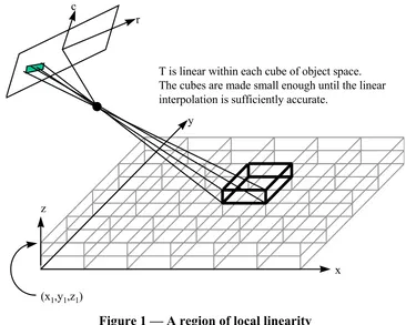
The accuracy of the grid interpolation image geometry is increased by using a smaller grid point spacing in object space. The rule is simple: Given a maximum error budget, choose the grid spacing so that the maximum error introduced by tri-linear interpolation is less than the error budget. Figure 1 is an illustration of the situation.

(x₁,y₁,z₁)

r c

x y

z

T is linear within each cube of object space. The cubes are made small enough until the linear interpolation is sufficiently accurate.

Figure 1 — A region of local linearity

5.5 Size of image support data

If the rigorous image geometry model has only low order components, only a modest number of grid points may be needed. Because optical projection can be accurately represented by ratios of first order polynomials, they have slowly changing (first order) partial derivatives. Furthermore, second order polynomials can accurately approximate many of the corrections used in rigorous models, such as for earth curvature, atmospheric refraction, and lens distortion. These correction functions thus have slowly changing

(13)

OGC 04-071

partial derivatives. When this is true, a grid that is small enough to be easily handled can also be fine enough to support a small error budget.

However, some image geometry models have high order model components. For example, camera vibration during the sweep of a panoramic camera can have tens of vibration cycles during the exposure of one image. If the peak-to-peak magnitude of the vibration or another high order effect is significantly larger than the desired maximum fitting error, then hundreds of grid points can be required in each of the three ground coordinates.

Since the (

x

i,

y

j,

z

k) grid points are equally spaced, the set of ground coordinates can be represented as a very small set of data. For example, each image point position might be represented by two short unsigned integers, with the row and column each having a range from 0 or 1 to the number of rows or columns in the image. Also, each ground point position might be represented by three short unsigned integers, by using an origin and point spacing for each coordinate.

5.6 Tri-linear interpolation mathematics

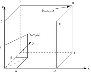
Tri-linear interpolation is relatively easy to compute. Assume that we are interpolating the function T within the grid cell with corners numbered from 1 to 8 as shown in Figure 2. Assume that T(xi,yi,zi) = (ri,ci) for i = 1, 2, …, 8, and the eight points (xi,yi,zi) are the

corners of the grid cell in object space. Further assume that (x0,y0,z0) is a point within the

polyhedron defined by the eight corners. The goal is to compute T(x0,y0,z0).

1 2

3

4 5

6

7 ₈

(x8,y8,z8)

α β γ

(x0,y0,z0)

x z

y

(14)

We first compute the parameters α, β, and γ using the equations:

α = (x0-x1)/(x2-x1) β = (y0-y1)/(y3-y1) γ = (z0-z1)/(z5-z1)

We then compute T at (x0,y0,z0) by:

T(x0,y0,z0) = (1-γ){(1-β)[(1-α)(r1,c1) + α(r2,c2)] + β[(1- α)(r3,c3) + α(r4,c4)]} + γ β)[(1- α)(r5,c5) + α(r6,c6)] + β[(1- α)(r7,c7) + α(r8,c8)]}

Using this formulation, the interpolation of T at an arbitrary point, takes 23 adds, 3 divides, and 20 multiplies, and can be further accelerated by careful implementation.

5.7 Advantages and disadvantages

The primary disadvantage of a Grid Interpolation Image Geometry Model is that the image support data will be very large when a large number of grid points are required. This situation normally occurs for certain image sensors having high order geometric effects, such as significant vibration during image collection and electronic array non-linearities. The advantages of a grid interpolation image geometry model include:

a) One grid model can be used for all types of images.

b) An exploitation system or software using the grid model can be completely ignorant of the rigorous image geometry model used to create it. The rigorous image geometry model is thus easier to update as sensors evolve, since changes to it do not cascade into the exploitation software. Configuration management of rigorous image geometry models is easier.

c) The same grid model can be used by all exploitation software, producing the same errors and error estimates in each. This commonality will make enterprise wide error analysis easier.

d) Transfer of image support data for this grid model can be robust, if the ground coordinates of each grid point are separately recorded. The loss of a few points in the set of 5-tuples is easy to detect by the obvious loss of symmetry, and is easy to patch (with some loss of accuracy) by interpolating or extrapolating from surviving points.

6 Ratios of polynomials

In the last few years, a Ratios of Polynomials approximate image geometry model has come into use, sometimes termed the Rational Functions model. The polynomial

coefficients for this model are sometimes called Rapid Positioning Capability (RPC) data. The image distribution agency computes the RPC data for each image, and distributes this data with the images.

(15)

OGC 04-071

6.2 Ratios of polynomials mathematics

This image geometry model uses a ratio of two polynomial functions to compute image row, and a similar ratio to compute image column. All four polynomials are functions of three ground coordinates, namely latitude, longitude, and height (or elevation). A

separate image geometry model is computed for each previously defined segment of a large image. Each polynomial has 20 terms, although the coefficients of some polynomial terms are often zero. In the polynomial functions, the three ground coordinates and two image coordinates are each offset and scaled to have a range from -1.0 to +1.0 over an image segment.

For each image or previously defined image segment, the defined ratios of polynomials have the form:

c

n = Normalized column index of pixel in image

x

n

, y

n

, z

n = Normalized ground coordinate values

The polynomials p and q have the form:

p

=

a

_ijk

x

ni

aijk

,

bijk

The maximum powers of each ground coordinate (m1, m2, m3, n1, n2, and n3) are limited to 3. Furthermore, the total power of all three ground coordinates is limited to 3. That is, the polynomial coefficients are defined to be zero whenever i + j + k > 3.

6.3 Normalized Ground Coordinates

(16)

normalized ground coordinates are computed from the un-normalized coordinates using the equations:

x

n

=

x

u

−

x

o

x

s

y

n

=

y

u

−

y

o

y

s

z

n

=

z

u

−

z

o

z

s

Where:

x

n,

y

n,

z

n = Normalized ground coordinate values

x

u,

y

u,

z

u = Un-normalized ground coordinate values, such as longitude, latitude, and height

x

o,

y

o,

z

o = Offset values for three ground coordinates

x

s,

y

s,

z

s = Scale factor values for three ground coordinates

The quantities

z

u,

z

o, and

z

s are all in the same units, normally meters. Similarly, the quantities

x

u,

y

u,

x

o,

y

o,

x

s, and

y

s are all in the same units, perhaps degrees of latitude and longitude.

6.4 Un-Normalized Image Coordinates

The row and column image coordinates (r and c) computed by the ratios of polynomials are offset and scaled to fit the range from -1.0 to + 1.0. The un-normalized image coordinates are computed from the normalized coordinates using the equations:

r

u

=

r

n

* r

s

+

r

o

c

u

=

c

n

* c

s

+

c

o

Where:

r

u,

c

u = Un-normalized image coordinate values

r

n,

c

n = Normalized image coordinate values

r

o,

c

o = Offset values for two image coordinates

r

s,

c

s = Scale factor values for two image coordinates

The quantities

r

u,

c

u,

r

o,

c

o,

r

s, and

c

s are all in the same units, namely pixel spacings.

(17)

OGC 04-071

6.5 Advantages and disadvantages

The ratios of polynomials image geometry model has many of the advantages discussed above for the grid interpolation model, including:

a) One ratio of polynomials model can be used for all types of images.

b) An exploitation system or software using the ratio model can be completely ignorant of the rigorous image geometry model used to create it. The rigorous image geometry model is thus easier to update as sensors evolve, since changes to it do not cascade into the exploitation software. Configuration management of rigorous image geometry models is easier.

c) The same ratio model can be used by all exploitation software, producing the same errors and error estimates in each. This commonality will make enterprise wide error analysis easier.

However, this ratios-of-polynomials image geometry model has several limitations:

a) Limited accuracy in fitting to the associated rigorous image geometry model

b) Sometimes fit to a rigorous image geometry model with limited accuracy (e.g., not triangulated with several overlapping images)

c) Complex fitting process, to avoid a denominator polynomial function going to zero within the image segment extent (producing excessive errors)

d) Not provided with all images distributed by the distributing agency

7 Universal image geometry model

The “Universal Image Geometry Model” is an extension of the ratios of polynomials model, which also employs interpolation of high-order correction functions. Although the universal model is more complex, it offers the advantage of higher storage efficiency (or more data compression) for image support data. It offers higher storage efficiency by not requiring a very large number of polynomials or points to accurately fit the rigorous sensor models of sensors having high order geometric effects (such as sensor vibration effects)

This Universal Image Geometry Model is universal in the sense that we think it can accurately represent the geometry of all known types of images and image sensors. These image sensor types include frame, panoramic, pushbroom, whiskbroom, and Synthetic Aperture Radar (SAR) sensors. This model can accurately represent images from all these sensor types for purposes of image exploitation, but not for image geometry model adjustment, by triangulation and most other adjustment methods.

(18)

11.3 of the Fifth Edition of the Manual of Photogrammetry, published by the American Society of Photogrammetry and Remote Sensing in 2004. This Replacement Sensor Model is also described by documents now publicly available on the web page http://www.ismc.nga.mil/ntb/.

(19)

OGC 04-071

Bibliography

[1] OGC 96-012, An Interface for Earth Image Math Models, by Cliff Kottman

[2] OGC 97-003, A Universal Image Geometry Model, by Arliss Whiteside

[3] OGC 99-107, The OpenGIS™ Abstract Specification Topic 7: The Earth Imagery Case

[4] OGC 00-116, The OpenGIS™ Abstract Specification Topic 16: Image Coordinate Transformation Services

[5] OGC 02-006, OGC Abstract Specification Topic 6: The Coverage Type and its Subtypes, which contains ISO 19123

[6] ISO 19123, Geographic information — Coverage geometry and functions

[7] Manual of Photogrammetry, American Society of Photogrammetry, Fifth Edition, 2004

Discussion Papers | OGC

Open Geospatial Consortium Inc.

Some image geometry models

Contents

Figures

i. Preface

ii. Revision

history

Foreword

Some image geometry models

r

=

a

x

x

y

z

aijk

,

bijk

r

=

a

a

* x

+

a

* y

c

=

b

b

* x

+

b

* y

r

c

x

y

a

o

, a

x

, a

y

, b

o

, b

x

, b

y

x

y

z

x

y

z

x

y

z

x

y

z

c

x

, y

, z

p

=

a

x

aijk

,

bijk

x

=

x

−

x