AN INTERACTIVE WEB-BASED ANALYSIS FRAMEWORK FOR REMOTE SENSING
CLOUD COMPUTING
X. Z. Wang a1, H. M. Zhanga1, J. H. Zhao a, Q. H. Lin a, Y. C. Zhou a, J. H. Li a *
a Computer Network Information Center, Chinese Academy of Sciences, Beijing, China -
(wxz, hai, zjh, lqh, zyc, lijh)@cnic.cn
KEY WORDS: Spatiotemporal Cloud Computing, Distributed File System, Lightweight Container, IPython Notebook, Remote Sensing Data Analysis
ABSTRACT:
Spatiotemporal data, especially remote sensing data, are widely used in ecological, geographical, agriculture, and military research and applications. With the development of remote sensing technology, more and more remote sensing data are accumulated and stored in the cloud. An effective way for cloud users to access and analyse these massive spatiotemporal data in the web clients becomes an urgent issue. In this paper, we proposed a new scalable, interactive and web-based cloud computing solution for massive remote sensing data analysis. We build a spatiotemporal analysis platform to provide the end-user with a safe and convenient way to access massive remote sensing data stored in the cloud. The lightweight cloud storage system used to store public data and users’ private data is constructed based on open source distributed file system. In it, massive remote sensing data are stored as public data, while the intermediate and input data are stored as private data. The elastic, scalable, and flexible cloud computing environment is built using Docker, which is a technology of open-source lightweight cloud computing container in the Linux operating system. In the Docker container, open-source software such as IPython, NumPy, GDAL, and Grass GIS etc., are deployed. Users can write scripts in the IPython Notebook web page through the web browser to process data, and the scripts will be submitted to IPython kernel to be executed. By comparing the performance of remote sensing data analysis tasks executed in Docker container, KVM virtual machines and physical machines respectively, we can conclude that the cloud computing environment built by Docker makes the greatest use of the host system resources, and can handle more concurrent spatial-temporal computing tasks. Docker technology provides resource isolation mechanism in aspects of IO, CPU, and memory etc., which offers security guarantee when processing remote sensing data in the IPython Notebook. Users can write complex data processing code on the web directly, so they can design their own data processing algorithm.
* Corresponding author at: Computer Network Information Center, Chinese Academy of Sciences (CNIC, CAS), 4,4th South Street, Zhongguancun, P.O. Box 349, Haidian District, Beijing 100190, China. Tel.: +86 010 5881 2518.
E-mail address: [email protected] (J. Li).
1 These authors contributed equally to this work. 1. INTRODUCTION
With fast development of geospatial data generating technologies, vast quantities of geospatial data are accumulated in an enhanced way, especially the remote sensing data which are taken by sensors on satellites. Nowadays, thousands of man-made satellites are orbiting the earth (Martinussen et al., 2014), and images generated from those satellites have more bands and higher resolution. At the same time, a growing number of geospatial portal makes data retrieval, ordering and downloading possible for everyone, such as USGS Earth Explorer, European's Space Agency(ESA), Canada's Open Data portal, and GSCloud (Wang et al., 2015) etc. These work have benefited geoscientists tremendously and are transforming geosciences as well (Vitolo et al., 2015).
In traditional way, scientists use commercial or free software to analyze remote sensing data in their workstations. At first, scientists need to download or copy remote sensing data into their workstation, and then use related analysis tools or write scripts to process these data. It usually takes a lot of time. The dramatic increase in the volume of geospatial data availability has created many challenges. First, the fact that remote sensing data are inherently large significantly increases the complexity
of corresponding technologies related to data management and data analysis work. Moreover, many research fields require large time span and spatial coverage to do related work, especially environmental science. The sheer quantity of data poses technical difficulties for obtaining and processing. Thus, time-consuming and data intensive is steadily becoming the dominant challenge of geospatial data computing nowadays (Bryant et al., 2008). Second, with the computing demands increasing in massive geospatial data computing, a scientist’s personal computer or workstation will quickly be overwhelmed for its low computing speed. On the one hand, purchasing high-performance computing infrastructure is generally not cost-effective in aspects of money, power, space, people, and so on. On the other hand, all the computing infrastructure will quickly become outdated. So the resource deficiency greatly hinders the advancements of geospatial science and applications (Yang et al., 2011). Third, facing the large scale of massive geospatial data that beyond which the researchers have previously encountered, the traditional process method would not work. Researchers may have to design software architectures to accommodate the large volume of data (Li et al., 2010). As most work are under specific scientists, there is a chance that they do not have enough computing expertise. Thus, in the absence of suitable expertise and infrastructure, an apparently simple task
may become an information discovery and management nightmare (Foster et al., 2012).
The emergence of cloud computing greatly enhances the advancement of processing massive geospatial data in the Cloud (Cui et al., 2010, Huang et al., 2010). However, these applications are mainly concentrated in the interactive online visualization and batch processing analysis. For the most popular base maps (e.g., Google Maps, Bing Maps), remote sensing imagery is pre-processed and mosaicked at various zoom levels and cached into tiles that serve as background images. Another example in batch processing analysis is the global 30m map of forest cover and change from 2000-2012 (Hansen et al., 2013). Based upon analyses of massive quantities of Landsat data co-located in cloud storage, it quantifies forest dynamics related to fires, tornadoes, disease and logging, worldwide. The analyses required over one million hours of CPU and would have taken more than fifteen years to complete on a single computer. But because the analyses were run on 10,000 CPUs in parallel in the Google cloud infrastructure, they were completed in less than four days. As cloud computing technology continues to evolve, placing remote sensing data into the cloud, and providing online interactive analysis services become more feasible. Amazon Web Services just opened up Landsat on AWS, a publicly available archive of Landsat 8 imagery hosted on their reliable and accessible infrastructure, so that anyone can use Amazon’s computing resources (EC2 instances or EMR clusters) on-demand to perform analysis and create new products without worrying about the cost of storing Landsat data or the time required to download it (http://aws.amazon.com/cn/public-data-sets/landsat/). Although currently demo applications relies on these Landsat data mainly focused on the interactive online visualization, more interactive scientific analysis may be available in the future. These efforts greatly facilitates scientists to use these data for scientific analysis.
Remote sensing data is a typical geoscience data, the processing for these data has the following typical characteristics: data intensity, computing intensity, concurrent intensity and spatiotemporal intensity. In most cases, geoscience phenomena are complex processes and geoscience applications often take a variety of data types as input in a long and complex workflow (Yang et al., 2011). How to decompose and express these complex workflow in the cloud environment is a major challenge. General scientific workflow technology is usually considered to be a good solution for the expression of complex scientific model, and it has been widely used in many scientific research. By scientific workflow, scientists can model, design, execute, debug, re-configure and re-run their analysis and visualization pipelines (Goecks et al., 2010). Another solution for complex scientific problem is programming. Programming is more flexible and robust than scientific workflow, and it is able to solve more complex scientific computing. With the advent of the era of mobile office, an increasing number of scientific application migrate to the browser. How to implement the complex process of scientific data analysis in browser is a meaningful thing.
In this paper, a new scalable, interactive, web-based massive data processing environment based on Docker, IPython and some open source geosciences tools is proposed. It offers safer and much more convenient way for the end-user to access massive data resources in the cloud. Users can write data processing code on the web directly, so they can design their own data processing algorithm. The remainder of this paper is
structured as follows. Section 2 discusses the related works about spatiotemporal cloud computing, server virtualization and cloud-based scientific workflow system. Section 3 gives an overview of the methodology and system architecture. In section 4, we introduce the system implementation. Section 5 introduces experiments and performance analysis. In section 7 we conclude our work with discussions and discussed our future work.
2. RELATED WORK
Cloud computing is developed mainly by big internet-based companies such as Amazon, Google and Microsoft which make great investment in ‘mega-scale’ computational clusters and advanced, large-scale data storage systems (Schadt et al., 2010). Though these commercial cloud computing platforms are perceived for “business applications”, such as Amazon’s Elastic Compute Cloud, Google App Engine, and Microsoft’s Windows Azure, as they has the potential to eliminate or significantly lower many resource barriers and data barriers that have been existing for a long time in geoscience domain, they provide a cost-effective, highly scalable and flexible solution for those large-scale, compute- and data- intensive geoscience researches (Li et al., 2010).
Amazon’s management console – which can be accessed from any web browser – provides a simple and intuitive interface for several uses: moving data and applications into and out of the Amazon S3 storage system; creating instances in Amazon EC2; and running data-processing programs on those instances, including the analysis of big data sets using MapReduce-based algorithms. In EC2, users can customize the environment for their particular application by installing particular software or by purchasing particular machine images (Schadt et al., 2010). Windows Azure Cloud computing platform hides data complexities and subsequent data processing and transformation form end users, and it is highly flexible and extensible to accommodate different science data processing tasks, and can be dynamically scaled to fulfil scientists’ various computational requirements in a cost-efficient way. Li implemented a particular instance of a MODIS satellite data re-projection and reduction pipeline in the Windows Azure Cloud computing platform, and the experiment results show that using the cloud computing platform, the speed of large-scale science data processing can be 90 times faster than that on a high-end desktop machine (Li et al., 2010). The first global assessment of forest change at pixel scale has been completed under Google cloud environment in 2013(Hansen et al., 2013). It contains spatially and temporally detailed information on forest change based on Landsat data at a spatial resolution of 30m from 2000 to 2012. As it is definitely data- and compute- intensive application, personal computers or workstation cannot afford this computation work. Key to the project was collaboration with team members from Google Earth Engine, who reproduced in the Google Cloud the models developed at the University of Maryland for processing and characterizing the Landsat data (http://www.nasa.gov/audience/ forstudents/k-4/stories/what-is-a-satellite-k4.html). As a professional geoscience software, ENVI has also developed its first cloud-based remote sensing system, the ENVI and IDL Service Engine, on Amazon’s EC2 platform. It is an enterprise-enabled processing engine that provides remote users access to the power of ENVI image analysis and IDL applications form a web or mobile client interface (O’Connor et al., 2012).
Except all those commercial corporations, many scientists are putting more emphasis on how to apply cloud computing into geosciences. Cary try to combine cloud computing with spatial data storage and processing and solve two key problems by using MapReduce framework, an R-Tree index for all kinds of spatial data and remote sensing image quality evaluations (Cary et al., 2009). Blower implement a web map service on Google App Engine and describe the difficulties in developing GIS systems on the public cloud (Blower, 2010). Karimi study distributed algorithms for geospatial data processing on clouds and compared their experimentation with an existing cloud platform to evaluate its performance for real-time geoprocessing. (Karimi et al., 2011). Cloud computing has brought great breakthrough and innovation to the geosciences.
The essence of cloud computing is to provide users with computing resource. Resource management is critical in cloud computing. There are kinds of resources in the large-scale computing infrastructure need to be managed, CPU load, network bandwidth, storage quota, and even type of operating systems. In order to limit, isolate and measure the use of computing resources for each user, server virtualization is widely used to manage the resource in data centers. Virtualization is the key technology in cloud computing which allows systems to behave like a true physical computer, while with flexible specification of details such as number of processors, memory and disk size, and operating system (Schadt et al., 2010). All IT resources are turned into a service that customers can rent based on their practical need and team work through the internet. And cloud computing provides easy-to-use interfaces to domain specialists without advanced technical knowledge (i.e. meteorologists, geography specialists, hydrologists, etc.) to process massive geospatial data. In addition, it provides elastic and on-demand access to massively pooled, instantiable and affordable computing resources as well (Cui et al., 2010, Huang et al., 2010).
Figure 1. The difference between hypervisor and container architecture
Currently there have two wildly used virtualization technology: VM hypervisors and container (Figure 1). The key difference between containers and VMs is that while the hypervisor abstracts an entire device, containers just abstract the operating system kernel. VM hypervisors, such as Hyper-V, KVM, and Xen, are all based on emulating virtual hardware. That means they’re fat in terms of system requirements.
Docker, a new open-source container technology, is hotter than hot because it makes it possible to get far more apps running on the same old servers and it also makes it very easy to package and ship programs. Docker uses LXC, cgroups and Linux’s own kernel. Compared with traditional virtual machine, a Docker container does not contain a single operating system, but runs based on the functionality provided by operating system in the existing infrastructure. Docker's core is Linux cgroups (control group) which provides methods that compute and limit the
resources of CPU, memory, network, and disk that containers can use. Different from virtualized application which includes not only the application – which may be only 10s of MB – and the necessary binaries and libraries, but also an entire guest operating system – which may weigh 10s of GB, the Docker Engine container comprises just the application and its dependencies. Docker runs as an isolated process in user-space on the host operating system, sharing the kernel with other containers. Thus, it enjoys the resource isolation and allocation benefits of VMs but is much more portable and efficient.
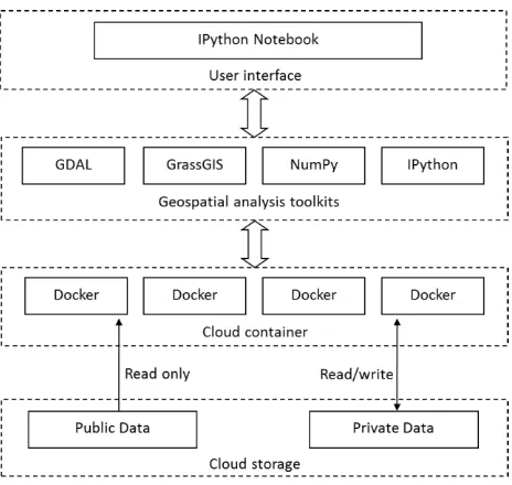
3. METHODOLOGY & SYSTEM ARCHITECTURE To provide interactive online analysis for remote sensing data, the overall system architecture of the cloud system needs to meet the following typical characteristics. First, a unified interactive data analysis interface is essential to implement long and complex spatiotemporal workflow. Second, a geospatial analysis toolkits deployed in the cloud environment provides abundant predefined and customized data analysis functions. Third, a lightweight cloud computing container performs execution of these spatiotemporal analysis tasks. Four, an efficient cloud storage environment stores public remote sensing data and user’s private data, and provides detailed access control. The architecture is depicted in Figure 2.
Figure 2. Overall system architecture
3.1 A Flexible User Interface
Geoscience applications often take a variety of data types as input with a long and complex workflow. Programming is more flexible and robust than traditional scientific workflow, and it is able to solve more complex scientific computing. As roots in academic scientific computing, IPython has become the most popular tool for maintaining, sharing, and replicating long science data workflows (Helen et al., 2014). IPython Notebook is a web-based interactive computational environment connecting to IPython kernel. IPython Nodebook allows customization and the flexibility of executing code in a live Python environment. Through this way, many complex scientific calculation, scientific drawing, parallel computing, and even Linux system shell call, can be realized by way of interacting on the network. In this paper, IPython Notebook was used as interactive analysis environment. Users write processing
scripts in the IPython Notebook, and interactively call geospatial analysis toolkits and system resources for remote sensing data analysis.
3.2 Geospatial Analysis Toolkits
Geospatial analysis toolkits include a variety of popular open-source spatiotemporal software, such as GDAL, Grass GIS, and scientific python distributions, such as NumPy and SciPy. The IPython kernel is the core component, which manages these software and provides public interface to IPython Notebook. These third-party software and python distributions can be used in two ways respectively to interact with IPython Kernel. One is that the python distributions can be directly imported as Python module into IPython project. The second way is that for the third-party software, IPython project can invoke system call to execute these external programs.
GDAL is a universal library for reading and writing raster and vector geospatial data formats. It provides a variety of useful command-line utilities for data translation and processing. With these GDAL utilities and IPython Notebook, users can perform some basic remote sensing processing and analysis, such as projection transformation, cutting and mosaic of remote sensing images. GDAL also provides python interface to directly access both raster and vector data. Grass GIS is an open source geographical information system capable of handling raster, topological vector, and image processing and graphic data. It also provides python interface to connect with IPython kernel.
3.3 An Lightweight Cloud Container
Previous studies (Huang et al., 2013) has shown that the generic cloud computing platforms, such as Amazon EC2 and Windows azure et al., cannot meet the requirements of complex geospatial cloud computing. To provide efficient and secure cloud computing environment to perform spatial analysis task, a lightweight cloud container Docker was used in this research. It runs as an isolated process in user-space on the host operating system, sharing the kernel with other containers. The IPython kernel and other geospatial analysis toolkits was packaged inside Docker’s virtual file system. Each Docker instance execute a single IPython kernel, which is responsible for receiving and processing requests from IPython Notebook.
3.4 An Secure and Stable Cloud Storage
Our system needs a stable and secure cloud storage file system to store public remote sensing data and the user’s private data. The data resources within the cloud storage can be accessed by IPython kernel inside Docker container. The cloud storage file system should have strict access control. For public data, it provides read-only privilege. Meanwhile, for user’s private data, it provides read/write privilege.
Table 1. The comparison of distributed file systems Fault
tolerance
Quota Web
GUI
Meta Data Server
Status
Ceph Yes Yes No Need Developing
Gluster Yes No Yes Not need Stable
MooseFS Yes Yes Yes Need Stable
Currently, distributed file system is the best cloud storage architecture to achieve these goals. The comparison between three famous open-source distributed file systems is listed in table 1. Quota control, high performance and stable are the key features of our system.
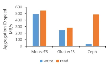
Figure 3. The aggregation IO speed comparison of three distributed file systems
In order to select an appropriate distributed file system, we tested the aggregation IO speed of three different distributed file system. The configuration of the test environment is listed in section 4. From the comparison of aggregation IO speed (Figure 3), we can find that MooseFS has higher aggregation IO speed, and it meets the requirements of cloud storage.
4. SYSTEM IMPLIMENTATIONS
The system is developed on the basis of open-source systems and software, such as Linux operating system (Fedora v21), MooseFS (v2.0), Docker (v1.3), IPython (v2.3), GDAL (v1.10) and Nginx (v1.7). The test environment includes 10 physical servers. These servers are connected through local area networks (LANs with 10Gbps). Each server has 32 GB memory, two Xeon E5-2620 six-core processors with a clock frequency of 2.00 GHz and 12*6TB SATA hard drivers.
4.1 Implementation of Cloud Storage
The cloud storage file system is constructed by MooseFS, and all data is stored in this file system. There have two types of data: public data and private data, which are stored under the directories of /public and /private respectively. The access permission of private data is read/write, while public data are restricted to read-only. For each user, the private data is stored in a separate folder under the /private directory. So all users’ private data storage space constitute a set of subdirectories under the /private directory in the cloud storage file system.
Figure 4. Data mapping mechanism
All the public data and private data are mounted to the Docker server through MooseFS mount client, under the directories of /mnt/public and /mnt/private respectively. When creating and
using a Docker container, a user can map the public directories and the private directories to corresponding Docker container through Docker management command. For example, the private data directory of user.1 in MoosFS is /private/user.1. The mapped directory in the container will be /mnt/private/user.1. The mapping mechanism is depicted in Figure 4.
4.2 Management of Docker Containers
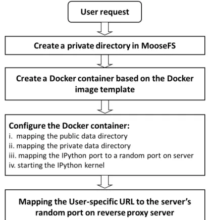
The creation process of Docker containers is depicted in Figure 5. When the system receives a new request to create new Docker container, the system automatically creates a private directory to store user’s private data. Before starting Docker container, we need to prepare a Docker image in advance. This Docker image is created base on the host server. In our test environment, the host server is installed with Fedora V21 Linux operate system. All the required software and toolkits, such as GDAL, Grass GIS, and IPython kernel etc., are pre-installed. We can create and launch Docker container through the following Docker command.
docker run -v /mnt/public:/mnt/public -v /mnt/private/subdirectory.1:/mnt/private -p 9001 -p 8888 -m 2g -c 100 -d 26c ipython notebook --profile=nbserver
After the command execution is complete, a Docker container is automatically created and IPython kernel and Notebook server is also started up. At the same time, the public and private data storage are mounted to corresponding cloud storage directory. And also the assigned port 8888 of IPython kernel server inside Docker container is also mapped to the corresponding port of the host server. This command also specifies the maximum amount of 2GB memory available to Docker container, and the relative maximum CPU utilization to 100.
Figure 5. The management process of Docker containers
The restriction of the container’s disk IO is implemented by changing the system attribute value, which is BlockIOReadBandwidth/BlockIOWriteBandwidth of the location where container’s file system are mounted in the host. For example, if we want to restrict the write speed to 10M, the command can be wrote as:
systemctl set-property --runtime docker-ID.scope "BlockIOWriteBandwidth=/dev/mapper/docker-ID 10M"
4.3 Access IPython Instances
When Docker container starts, the IPython kernel automatically start providing services on the binding port. The IPython binding port is mapped to the host server port which connects with two Nginx servers. Each IPython binding port are associated with a unique URL through reverse proxy in Nginx. The Route of access IPython instances is depicted in Figure 6. Just by logging in to dedicated IPython Notebook web page using user-specific URL in the web browser, users can access all the computing and data resources, upload and perform procedures, and view the results on line.
Figure 6. Route of access IPython instances
5. EXPERIMENTS AND ANALYSIS 5.1 Experiment Design
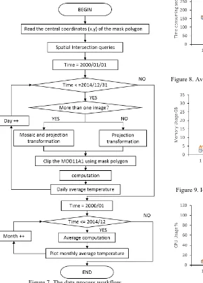
An experiment about long time series of monthly average land surface temperature of a given region from 2000 to 2014 are conducted to test the performance and reliability of this system, The region is defined by the mask data users upload. The monthly average land surface temperature is computed using MOD11A1, which is a kind of MODIS LST data products. The MOD11A1 product comprises the following Science Data Set (SDS) layers for day time and night time observations: LSTs, quality control assessments, observation times, view zenith angles, clear sky coverage, and bands 31 and 32 emissivity from land cover types (https://lpdaac.usgs.gov/products/modis_ products_table/mod11a1). In this experiment, only the LSTs data set are used as input parameter. The whole data process workflow is depicted as figure 4. Though the algorithm of computing monthly average temperature of a given region from MOD11A1 is simple, a lot of computing work are needed when managing and processing all of the data due to the long time period. During the whole process, MOD11A1 data are stored in public storage, while all the intermediate results data are stored in the user’s private storage space. The data process workflow includes 2 separate loop computations.
1) Daily average temperature computation
To compute the average land surface temperature of a region, users firstly have to upload the polygon data of the region, which is called mask polygon in this procedure. The projection of the mask polygon is WGS 84, and it can be in a shapefile or KML format. The central coordinate (x, y) is then obtained, which is used to perform intersection spatial queries to find those MOD11A1 images that contains the coordinate. In this experiment, the time period starts from 2000/01/01 to 2014/12/31. The MOD11A1 data are processed in units of days chronologically. Determine the number of those images that
cover the mask polygon every day. If there are more than one images, then mosaic is firstly operated, and then is the projection transformation which transforms the original sinusoidal projection into WGS 84. If there is only one MOD11A1 image covering the mask polygon, then only projection transformation is executed. Then the mask polygon is used to clip the mosaic or single MOD11A1 data. All of these calculations include cutting, mosaic, projection transformation could be done with a GDAL utilities named gdalwarp. When computing the daily average temperature for the study region, the Kelvin unit of temperature is firstly transformed into Degrees Celsius for ease of use according to the following formula: 0.02*value - 273.15. The daily average land surface temperature can be obtained by performing this simple formula in Python.
2) Monthly average temperature computation
After the daily average temperature are obtained, monthly average temperature are computed as well. And the monthly average temperature for each month from 2000 to 2014 is plotted as a line graph using the Python package PyPlot in the end. All the process can be implemented in the system introduced above using IPython with the user’s interaction.
Figure 7. The data process workflow
5.2 Performance Analysis
To test the performance of this system architecture in terms of system load and response efficiency, the core computing process of the aforementioned experiments were carried out in Docker, KVM and Physical machine respectively. Docker and KVM are installed in the same physical machine environment with configuration of that mentioned in section 4. Multi-task processes are executed concurrently when testing the physical environment. And different number of virtual machines are started on the physical machine at the same time when testing the KVM environment. The memory of each virtual machine is 2GB, and each virtual machine has one computing task running inside. As to the Docker environment test, different number of Docker are started in the physical machine, and each has one computing task running inside. Test indicators include the average time it takes to execute different concurrent tasks, memory consumption of physical machine, and CPU usage. Tests are performed under different concurrent tasks, and the results are shown in Figure 8, 9, and 10.
Figure 8. Average execution time of different concurrent tasks
Figure 9. Host memory usage of different concurrent tasks
Figure 10. Host CPU usage of different concurrent tasks
From the figures 8, 9, and 10, we can see that Docker and Host machine have little difference in terms of performance, as Docker containers share the resources of the physical machine environment. From the aspect of time-consuming, the average execution time increases with the increasing number of concurrent tasks, and the rate of increase is especially significant under KVM environment. In the host memory consumption aspect, the usage of memory and CPU increase with increasing number of concurrent tasks. Because each KVM virtual machine requires 2GB memory exclusively, the host memory will not be adequate when the number of virtual machine reaches 16. Since geosciences has the characteristics of computing-intensive, the CPU usage under the three tests do not differ greatly. To sum up, from the performance tests, we can see that the cloud environment based on Docker can maximize the utilization of the system resources, and thus can handle more concurrent spatial-temporal computing tasks.
6. CONCLUSIONS AND FUTURE WORK In this paper, we proposed a new scalable, interactive and web-based cloud computing solution for massive remote sensing data analysis. The lightweight cloud storage system used to store public data and users’ private data is constructed based on open source distributed file system. In it, massive remote sensing data are stored as public data, while the intermediate and input data are stored as private data. The elastic, scalable, and flexible cloud computing environment is built using Docker, which is a technology of open-source lightweight cloud computing container in the Linux operating system. In the Docker container, open-source software such as IPython, GDAL, and Grass GIS etc., are deployed. The cloud storage space is mounted inside the container, which makes it possible to access public and private data of the platform by IPython. Users can write scripts in the IPython Notebook page through the web browser to process data, and the code will be submitted to IPython kernel to be executed. Thus, massive remote sensing data processing in the Internet has been achieved.
By comparing the performance of remote sensing data analysis tasks executed in Docker container, KVM virtual machines and physical machines respectively, we can conclude that the cloud computing environment built by Docker makes the greatest use of the host system resources, and can handle more concurrent spatial-temporal computing tasks. Docker technology provides resource isolation mechanism in aspects of IO, CPU, and memory etc., which offers security guarantee when processing remote sensing data in the IPython Notebook.
In this paper, remote sensing data are processed based on IPython Notebook, which requires the users to be proficient in Python. However, this is a great obstacle for those scientists who has never used this language. So how to combine scientific workflow with IPython will be the focus of future work. Thus, user can drag and drop workflow controls on the web page to construct scientific workflow, then, the system will parse the workflow into IPython scripts automatically and the scripts will be submitted to IPython kernel to be executed. Remote sensing data processing is a typical data- and computing- intensive work. How to integrate parallel computing, multi-core technology, and clustering technology to improve data processing efficiency in IPython is a subject need to be studied in the future.
ACKNOWLEDGEMENTS
This work is supported by “Twelfth Five-Year” Plan for Science & Technology Support under Grant No. 2012BAK17B01 and 2013BAD15B02, the Natural Science Foundation of China (NSFC) under Grant No.91224006, 61003138 and 41371386, the Strategic Priority Research Program of the Chinese Academy of Sciences under Grant No. XDA06010202 and XDA05050601, and Youth Innovation Promotion Association of CAS (2014144).
REFERENCES
Blower, J. D., 2010. GIS in the cloud: implementing a Web Map Service on Google App Engine. In Proceedings of the 1st International Conference and Exhibition on Computing for Geospatial Research & Application, ACM, pp 34.
Bryant, R., Katz, R. H., & Lazowska, E. D., 2008. Big-data computing: creating revolutionary breakthroughs in commerce, science and society, 1-15.
Cary, A., Sun, Z., Hristidis, V., & Rishe, N., 2009. Experiences on processing spatial data with mapreduce. In Scientific and Statistical Database Management, Springer: Berlin Heidelberg, pp 302-319.
Cui, D., Wu, Y., & Zhang, Q., 2010. Massive spatial data processing model based on cloud computing model. In 2010 Third International Joint Conference on Computational Science and Optimization (CSO) 2, IEEE, pp 347-350.
Deelman, E., Singh, G., Livny, M., Berriman, B., & Good, J., 2008. The cost of doing science on the cloud: the montage example. In Proceedings of the 2008 ACM/IEEE conference on Supercomputing (p. 50). IEEE Press. 2013. High-resolution global maps of 21st-century forest cover change. Science, 342(6160), 850-853.
Shen H., 2014. Interactive notebooks: Sharing the code. Nature, 515 (7525): 151–152.
Huang, Q., Yang, C., Nebert, D., Liu, K., & Wu, H., 2010. Cloud computing for geosciences: deployment of GEOSS clearinghouse on Amazon's EC2. In Proceedings of the ACM SIGSPATIAL International Workshop on High Performance and Distributed Geographic Information Systems, pp 35-38.
Karimi, H. A., Roongpiboonsopit, D., & Wang, H., 2011. Exploring Real‐Time Geoprocessing in Cloud Computing: Navigation Services Case Study. Transactions in GIS, 15(5), 613-633.
Li, J., Humphrey, M., Agarwal, D., Jackson, K., van Ingen, C., & Ryu, Y., 2010. escience in the cloud: A modis satellite data reprojection and reduction pipeline in the windows azure platform. In Parallel & Distributed Processing (IPDPS), 2010 IEEE International Symposium on. IEEE. Pp 1-10
Martinussen, E. S., Knutsen, J., & Arnall, T., 2014. Satellite lamps. Inventio.
O’Connor, A., Lausten, K., Okubo, B., & Harris, T., 2012. ENVI Services Engine: Earth and planetary image processing for the cloud. American Geophysical Union, Poster IN21C-1490.
Huang Q., Yang C., Benedict K., Chen S., Rezgui A. and Xie J., 2013. Utilize cloud computing to support dust storm forecasting. International Journal of Digital Earth, 6(4), pp. 338-355.
Schadt, E. E., Linderman, M. D., Sorenson, J., Lee, L., & Nolan, G. P., 2010. Computational solutions to large-scale data management and analysis. Nature Reviews Genetics, 11(9), 647-657.
Vitolo, C., Elkhatib, Y., Reusser, D., Macleod, C. J., & Buytaert, W., 2015. Web technologies for environmental Big Data. Environmental Modelling & Software, 63, 185-198.
Wang X., Zhao J., Zhou Y., & Li J., 2014. The Geospatial Data Cloud: An Implementation of Applying Cloud Computing in Geosciences. CODATA: Data Science Journal. 13: 254-264
Yang, C., M. Goodchild, Q. Huang, D. Nebert, R. Raskin, Y. Xu, M. Bambacus, and D. Fay., 2011. Spatial Cloud Computing: How Could Geospatial Sciences Use and Help to Shape Cloud Computing. International Journal on Digital Earth, 4 (4): 305-329.