LOW-COST 3D LASER SCANNING IN AIR OR WATER USING SELF-CALIBRATING
STRUCTURED LIGHT
Michael Bleiera, Andreas N¨uchtera,b
a
Zentrum f¨ur Telematik e.V., W¨urzburg, Germany - [email protected]
bInformatics VII – Robotics and Telematics, Julius Maximilian University of W¨urzburg, Germany - [email protected]
Commission II
KEY WORDS:underwater laser scanning, structured light, self-calibration, 3D reconstruction
ABSTRACT:
In-situ calibration of structured light scanners in underwater environments is time-consuming and complicated. This paper presents a self-calibrating line laser scanning system, which enables the creation of dense 3D models with a single fixed camera and a freely moving hand-held cross line laser projector. The proposed approach exploits geometric constraints, such as coplanarities, to recover the depth information and is applicable without any prior knowledge of the position and orientation of the laser projector. By employing an off-the-shelf underwater camera and a waterproof housing with high power line lasers an affordable 3D scanning solution can be built. In experiments the performance of the proposed technique is studied and compared with 3D reconstruction using explicit calibration. We demonstrate that the scanning system can be applied to above-the-water as well as underwater scenes.
1 INTRODUCTION
The sea is becoming an increasingly important resource for the energy production industry and for mining of raw materials. In order to ensure the safe and efficient operation of structures, such as offshore wind turbines, oil platforms, or generators frequent inspections are necessary. High-resolution 3D scanners enable low-cost monitoring of submerged structures. Moreover, marine biologists have a strong interest in underwater 3D data acquisi-tion for the exploraacquisi-tion of ocean habitats. For example, the de-velopment of coral reefs is an important indicator of the well-being of the marine ecosystem. Having accurate measurements of the structural complexity of corals gives scientiests an indica-tor of the genetic diversity and spreading of diseases (Burns et al., 2015). Simple, low-cost 3D underwater sensors can have a significant impact on our ability to study the oceans.
For many underwater mapping applications sonar technology is still the primary solution because of its large sensor range and its robustness to turbidity. However, certain measurement tasks require a higher accuracy and resolution. For example, geolo-gists are interested in monitoring changes in lake bed sediments of small areas in flat water zones with sub-centimeter resolu-tion to create and verify detailed geotechnical models. Such re-quirements make optical scanners interesting despite their lack of range due to the high absorption of light in water. Today, low-cost action cameras provide easy access to suitable technol-ogy for acquiring underwater images and videos. Subsequently, photogrammetry has become a popular technique for creating 3D models of submerged environments and has been applied to di-verse scientific and industrial applications, such as marine ecosys-tem monitoring (Burns et al., 2015), non-destructive documenta-tion of archaeological sites (Drap et al., 2007), or surveys of ship accidents (Menna et al., 2013).
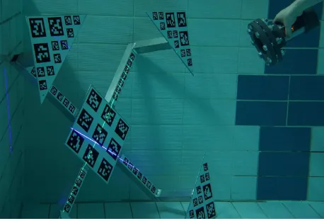
In this paper we propose a line laser scanning system consisting of a single camera and a hand-held cross line laser projector as depicted in Fig. 1. We employ a green and a blue line laser since absorption in water is significantly lower for these wavelengths than, for example, a red laser. Two different colors are employed to facilitate separation of the two laser lines in the camera image.
Figure 1: Cross line laser projector in a waterproof housing for underwater scanning.
The proposed approach is self-calibrating and is applicable with-out knowledge of the position of the projector in 3D space. Our method is based on self-calibration techniques proposed by Fu-rukawa and Kawasaki (2009), which exploit coplanarity and or-thogonality constraints between multiple laser planes to recover the depth information. We show that these results can be also adapted to underwater imaging.
The proposed system can be seen as a trade-off between pho-togrammetry and calibrated line laser scanning. Compared to photogrammetry the advantage is that operation in darkness and scanning of texture-less objects is possible. The restriction is that the self-calibration method is not applicable to completely planar scenes. However, in practice this is rarely a limitation because the approach can be applied to scenes with small depth variation.
The main drawback of explicit calibration is that the process has to be repeated every time a parameter is changed. This is chal-lenging in underwater environments, because it is difficult to work with calibration targets in water, e.g., divers can become neces-sary to move the calibration fixture or the scanner. This means that it takes a long time to capture a sufficient amount of low noise data that is suitable to perform system calibration. Therefore, au-tomatic parameter estimation techniques are of particular interest for being able to adapt the system to the environment without the need to re-calibrate.
In general, uncalibrated scanning with the projector moving with-out restrictions makes it more difficult to obtain accurate scans due to noisy estimates of the laser plane parameters. However, the accuracy of triangulation based depth estimation is also de-pendent on the baseline. Uncalibrated Structured Light has the advantage that we are not limited to a fixed distance and scanning with very large baselines becomes possible. A suitable baseline which depends on the depth range of the scene can be chosen by simply moving further away from the camera. This allows one to record details that would otherwise not show up in scans with a fixed small baseline.
2 RELATED WORK
In air conditions various techniques for inexpensive 3D scanning are available. Especially consumer RGB-D cameras, such as the Microsoft Kinect, had an important impact on low-cost 3D data acquisition. Coded structured light scanners using off-the-shelf digital projectors are capable of scanning small to medium size scenes with sub-millimeter precision (Salvi et al., 2004). Line laser scanning based on online calibration using markers or struc-tures in the scene, such as known reference planes (Winkelbach et al., 2006) or frames (Zagorchev and Goshtasby, 2006), is a pop-ular technique for scanning small objects. For larger distances a low-cost alternative to terrestrial 3D laser scanning based on a time-of-flight laser distance meter and a pan-and-tilt unit ex-ists (Eitel et al., 2013). For underwater applications the situation is different since most commercially available 3D range sensors are designed for atmospheric operation and do not work underwa-ter. Moreover, many industrial grade underwater sensing equip-ment is designed for subsea operation and water depths of more than 2000 m, which adds significantly to the costs. A comprehen-sive survey of optical underwater 3D data acquisition technolo-gies can be found in (Massot-Campos and Oliver-Codina, 2015).
2.1 Underwater Laser Scanning
The popularity of RGB-D cameras also inspired researchers to apply them to underwater imaging (Digumarti et al., 2016). How-ever, due to the infrared wavelength of the laser pattern projector the achievable range is limited to less than 30 cm (Dancu et al., 2014). Fringe projection has been applied successfully to acquire very detailed scans with high precision of small underwater ob-jects (T¨ornblom, 2010; Br¨auer-Burchardt et al., 2015). Despite the limited illuminating power of a standard digital projectors, working distances of more than 1 m have been reported in clear water (Bruno et al., 2011).
Commercial underwater laser scanning systems with larger mea-surement range often employ high-power line laser projectors. For example, scanners from “2G Robotics” offer a range of up to 10 m depending on the water conditions (2G Robotics, 2016). 3D scans are typically created by rotating the scanner and mea-suring the movement using rotational encoders or mounting the scanner to a moving platform and recording the vehicle trajectory data from inertial navigation systems and GNSS.
Recently, researchers employed diffractive optical elements and more powerful laser sources to project multiple lines or a grid for one shot 3D reconstruction (Morinaga et al., 2015; Massot-Campos and Oliver-Codina, 2014). In this work we choose delib-erately a more simple cross laser pattern because in the presence of water turbidity or reflections we expect that the laser lines can be segmented more robustly compared to grid patterns. More-over, with multi line or grid projectors the laser light is spread over a large surface area which requires a higher illuminating power to achieve the same depth range.
Most of the commercially available underwater laser range sen-sors are based on laser stripe projection or other forms of struc-tured light. More recently companies started development of time-of-flight underwater laser scanners. For example, the com-pany “3D at Depth” developed a commercial underwater LiDAR, which can be mounted on a pan-an-tilt unit to create 3D scans of underwater environments similar to terrestrial laser scanning (3D at Depth, 2016). A recently proposed scanning system by Mit-subishi uses a dome port with the scanner aligned in the optical center to achieve a wider field of view (Imaki et al., 2017).
2.2 Self-calibrating Line Laser Scanning
Exploiting the projection of planar curves on surfaces for recov-ering 3D shape has been studied for diverse applications, such as automatic calibration of structured light scanners (Furukawa et al., 2008), single image 3D reconstruction (Van den Heuvel, 1998) and shape estimation from cast shadows (Bouguet et al., 1999). In this section we focus on uncalibrated line laser scan-ning. Typically, these methods either employ a fixed camera and try to estimate the plane parameters of the laser planes or work with a setup where camera and laser are mounted rigidly relative to each other and their relative transformation needs to be esti-mated for calibration.
Some methods solve the online calibration problem by placing markers or known reference planes in the scene (Winkelbach et al., 2006; Zagorchev and Goshtasby, 2006). In contrast, Furukawa and Kawasaki (2006) proposed a self-calibration method for mov-able laser planes observed by a static camera that does not require placing any specific objects in the scene. The approach exploits coplanarity constraints from intersection points and additional metric constraints, e.g., the angle between laser planes, to per-form 3D reconstruction. It was demonstrated that 3D laser scan-ning is possible with a simple cross line laser pattern. Later, Fu-rukawa and Kawasaki (2009) extended the approach and showed how additional unknowns, such as, the parameters of a pinhole model (without distortion), can be estimated if a suitable initial guess is provided.
The plane parameter estimation problem leads to a linear sys-tem of coplanarity constraints for which a direct least-squares ap-proach does not necessarily yield a unique solution. For example, projecting all points of all planes in the same common plane ful-fills the coplanarity constraints. However, this does not reflect the real scene geometry. Ecker et al. (2007) showed how additional constraints on the distance of the points from the best fitting plane can be incorporated to avoid such unmeaningful solutions.
Object Figure 2: Cross line laser projector with a single fixed camera.
3 METHODOLOGY
The scanning setup for creating a 3D scan is visualized in Fig. 2. We scan the scene with a fixed camera and move the hand-held laser projector in order to project laser crosses in the scene from different 6 degrees of freedom poses. We explicitly calibrate the camera parameters, because this allows one to acquire robust esti-mates of the distortion parameters which are especially necessary for underwater imaging and uncorrected optics.
By aggregating a sequence of images over time, we can extract many different laser curves on the image plane. Since the camera is fixed we can find intersection points between the laser curves which correspond to the same 3D point. By extracting many laser curves, we will obtain many more intersection points than the number of laser planes. This allows us to exploit the intersections to estimate the plane parameters. However, from the intersection points alone we cannot solve all degrees of freedom (DOF) of the plane parameters. Using the additional orthogonality constraint between two laser planes in the cross configuration we can find the plane parameters up to an arbitrary scale. The 3D point posi-tions of each laser curve can then be computed by intersecting the camera rays with the laser plane. Outliers in this initial 3D recon-struction from inaccurately estimated laser planes are rejected by geometric consistency checks to create the final 3D point cloud.
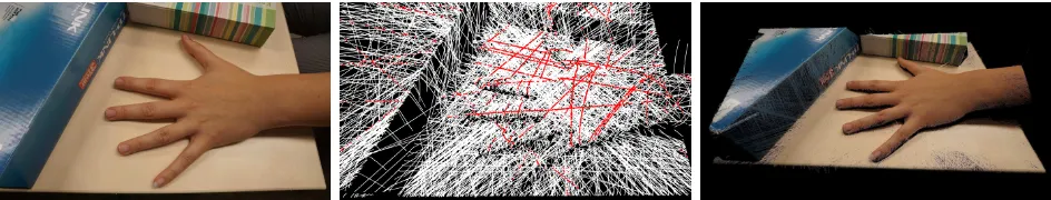
Fig. 3 shows an image of the scene captured from the perspective of the fixed camera used for scanning, a subset of the extracted laser curves in white and the computed intersection points in red, and the reconstructed 3D point cloud. This result was created from 3 min of video recorded at 30 fps. A total of 7,817 valid laser curves were extracted with 1,738,187 intersection points. The 3D reconstruction was computed using a subset of 400 laser planes. The final point cloud created from all valid laser curves has a size of 11,613,200 points. The individual steps and em-ployed models are explained in more detail in the following sec-tions.
3.1 Camera Model
We approximate the camera projection function based on the pin-hole model with distortion. Although in underwater conditions this model does not explicitly model the physical properties of refraction, it can provide a sufficient approximation for underwa-ter imaging and low errors are achievable (Shortis, 2015).
The pointX= (X, Y, Z)T
in world coordinates is projected on the image plane according to
(X, Y, Z)T 7−→(fxX/Z+px, fyY /Z+py)T= (x, y)T , (1)
wherex = (x, y)T
are the image coordinates of the projection, p= (px, py)Tis the principal point andfx,fyare the respective focal lengths. Using the normalized pinhole projection
xn=
we include radial and tangential distortion defined as follows
˜ distortion parameters. Here,x˜ = (˜x,y)˜ are the real (distorted) normalized point coordinates andr2=x2n+y2n.
We calibrate the camera using Zhang’s method (Zhang, 2000) with a 3D calibration fixture, see Fig. 1, with AprilTags (Olson, 2011) as fiducial markers. This has the advantage that calibra-tion points can be extracted automatically even if only part of the structure is visible in the image. In general, a larger calibration structure is beneficial especially in water since it can be detected over lager distances, which allows one to take calibration data in the whole measurement range. Moreover, it is known from lit-erature that 3D structures provide more consistent and accurate calibration results (Shortis, 2015).
After low level laser line extraction we undistort the image co-ordinates of the detected line points. Therefore, we do not have to consider distortion effects during the 3D reconstruction step, which simplifies the equations.
3.2 Laser Line Extraction
A simple approach to extracting laser lines from an image is to use maximum detection along horizontal or vertical scanlines in the image. In the case of uncalibrated scanning this does not work in all cases since the orientation of the laser line in the image is arbitrary and no clear predominant direction exists. Therefore, we employ a ridge detector for the extraction of the laser lines in the image. For this work we use Steger’s line algorithm (Steger, 1998).
The idea of the algorithm is to find curves in the image that have in the direction perpendicular to the line a characteristic 1D line profile, i.e., a vanishing gradient and high curvature. We apply the line detector to a gray image created by averaging the color channels. If scans are capture in strong ambient illumination, we apply background subtraction to make the laser lines more discriminable from the background.
The direction of the line in the two dimensional image is esti-mated locally by computing the eigenvalues and eigenvectors of the Hessian matrix wheregσ(x, y)is the 2D gaussian kernel with standard devia-tionσ,I(x, y)is the image andrxx,rxy,ryx,ryyare the partial derivatives. The direction perpendicular to the line is the eigen-vector(nx, ny)Twithk(nx, ny)Tk2 = 1corresponding to the eigenvalue with the largest absolute value. For bright lines the eigenvalue needs to be smaller than zero.
Figure 3: Visualization of the scene, extracted laser curves, and 3D point cloud. Left: Image of the scene from the perspective of the fixed camera used for scanning, Middle: Visualization of a subset of the extracted laser curves in white and intersection points in red, Right: Colored 3D point cloud.
where the first derivative in the direction perpendicular to the line vanishes with sub-pixel accuracy:
(qx, qy)T =t(nx, ny)T , (5)
where
t=− rxnx+ryny
rxxn2x+ 2rxynxny+ryyn2y
. (6)
Here, rx = ∂gσ∂x(x,y) and ry = ∂gσ∂y(x,y) are the first partial derivatives.
For valid line points the position must lie within the current pixel. Therefore,(qx, qy)∈[−0.5,0.5]×[−0.5,0.5]is required. Indi-vidual points are then linked together to line segments based on a directed search.
The response of the ridge detector given by the value of the max-imum absolute eigenvalue is a good indicator for the saliency of the extracted line points. Only line points with a sufficiently high response are considered.
To distinguish between the two laser lines we use the color in-formation and apply thresholds in the HSV color space. This is implemented using look up tables to speed up color segmentation. We apply only very low thresholds for saturation and brightness of the laser line. Depending on the object surface the laser lines can be barely visible and appear desaturated in the image.
3.3 3D Reconstruction Using Light Section
A line laser can be considered as a tool to extract points on the image plane that are projections of object points that lie on the same plane in 3D space. We describe the laser planeπiusing the general form
πi: aiX+biY +ciZ= 1 , (7)
where(ai, bi, ci)are the plane parameters andX= (X, Y, Z)T is a point in world coordinates. Using the perspective camera model described in Eq. 1 this can be expressed as
πi: ai
x−px
fx
+bi
y−py
fy
+ci=
1
Z , (8)
wherex= (x, y)T
are the image coordinates of the projection of Xon the image plane,p= (px, py)T is the principal point and
fx,fyare the respective focal lengths.
If we know the plane and camera parameters, we can compute the coordinates of a 3D object point X = (X, Y, Z)T
on the plane from its projection on the image plane x = (x, y)T by
intersecting the camera ray with the laser plane:
Z= 1
aix−fpx x +bi
y−py fy +ci
X=Zx−px fx
Y =Zy−py fy
.
(9)
3.4 Estimation of Plane Parameters Using Coplanarity and Orthogonality Constraints
From the recorded sequence of images the laser curves are ex-tracted as polygonal chains. We find the points that exist on mul-tiple laser planes by intersecting the polylines. This computation can be accelerated by spatial sorting, such that only line segments that possibly intersect are tested for intersections. Moreover, we can simplify the polylines to reduce the number of line segments. However, we need to do this with a very low threshold (less than half a pixel) in order not to degrade the accuracy of the extracted intersection positions.
The plane parameters are estimated in a two step process based on the approach described in (Furukawa and Kawasaki, 2009). First, by solving a linear system of coplanarity constraints the laser planes are reconstructed up to 4-DOF indeterminacy. Sec-ond, further indeterminacies can be recovered from the orthogo-nality constraints between laser planes in the cross configuration in a non-linear optimization.
Using Eq. 8 the coplanarity constraint between two laser planes
πiandπjcan be expressed in the perspective system of the cam-era for an intersection pointxij= (xij, yij)Tas
1 Zi(xij, yij)
− 1
Zj(xij, yij)
=
(ai−aj)
xij−px
fx
+ (bi−bj)
yij−py
fy
+ (ci−cj) = 0 .
(10)
We combine these linear equations in a homogeneous linear sys-tem:
Av= 0 , (11)
wherev= (a1, b1, c1, . . . , aN, bN, cN)Tis the combined vector of the planes’ parameters andAis a matrix whose rows contain
±(xij−px)fx−1,±(yij−px)fx−1and±1at the appropriate columns to form the linear equations of Eq. 10.
A degenerate condition can be caused, e.g., by planes with only collinear intersection points. The solution can be represented by an arbitrary offsetoand an arbitrary scales:
(a, b, c) =s(ap, bp, cp) +o . (12) With the cross line laser configuration we obtain an additional perpendicularity constraints between each of the two cross laser planes which can be used to recover the offset vector. The offset is computed, such that the error of the orthogonality constraints is minimized. We find the offset vectorˆothat minimizes the sum of the inner product between planes in the setC={(i, j)|(πi⊥
πj)}of orthogonal laser planes:
ˆ
wherenis the normal of the plane computed from the plane pa-rameters and offset vector. The scale cannot be recovered with only two laser planes and needs to be estimated from other mea-surements, such as a known distance in the scene.
We only use a subset of the laser planes to solve for the plane parameters. The other planes can then be reconstructed by fitting a plane to the intersection points with planes of the already solved subset of laser planes. Although it is possible to compute 3D reconstruction with less planes we found empirically that 100 -200 planes are necessary to find a robust solution.
In order to choose a solvable subset of planes we remove all planes that have only collinear intersection points. Moreover, we apply heuristics to select planes that have distinct orientations and positions in the image. To do this we pick planes spread apart in time. Consecutive frames can be very similar if we move the pro-jector slowly. Additionally, we reject planes that have more than one intersection with each other. There are situations where it is valid that two planes have multiple intersections. However, in practice this mostly happens for identical planes or due to erro-neous or noisy intersection detections.
It is difficult to verify that a valid 3D reconstruction is found. We cannot tell if the solution is valid by only looking at the residuals of Eq. 11 and Eq. 13 since we are optimizing for these values and they are expected to be small. Therefore, we look at the error of the planes that we did not take in the plane parameter optimiza-tion step. Specifically, we compute the root-mean-square angular error for all orthogonal laser planes.
3.5 Outlier Rejection
In practice the estimated plane parameters are noisy. The ex-tracted positions of the laser line points have some error or wrong laser curves can be detected in the image due to reflections. This leads to noisy positions of the intersection points or erroneous de-tected intersections. Therefore, there will be some outliers in the created 3D point cloud.
To reduce these effects we reject laser segments or the informa-tion from the complete plane based on the following three crite-ria: Firstly, we remove planes with a very small baseline (distance to the optical center of the camera) because these measurements can only provide a low accuracy. Planes with intersection points that fulfill the coplanarity constraints only with a large error are rejected as well. Secondly, we compare the 3D points recon-structed from the current plane for geometric consistency with the points from other planes. Planes that have many points with a large distance from their neighbor points reconstructed from other planes are removed. Thirdly, planes with points outside the expected measurement range are rejected.
4 EXPERIMENTS
For the experiments in air a consumer digital camera with an APS-C sized sensor and a wide angle lens with a focal length of 16 mm is used. The underwater scans are captured using a GoPro action camera. We record video at 30 fps in Full-HD res-olution (1920 x 1080 pixels). A high shutter speed is beneficial since we move the laser by hand. An exposure time in the range of 5 ms to 10 ms was used in the experiments in order to reduce motion blur. The projector is built from two 450 nm and 520 nm line lasers with a fan angle of 90◦
and an adjustable output power of up to 40 mW. Note that the fan angle is reduced in water to approximately 64◦
. We set the laser focus such that the line is as thin as possible over the whole depth range of the scene. Al-though this setup worked well in our experiments for scanning in turbid water a higher laser power and smaller fan angle is desir-able.
4.1 Comparison with Explicit Plane Parameter Estimation
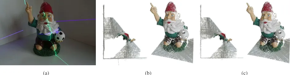
To verify the plane parameter estimation we compare the pro-posed approach with an explicit online calibration of the laser plane parameters using known reference planes in the scene. The setup is inspired by the David Laser Scanner (Winkelbach et al., 2006). We place three planes around the object as shown in Fig. 4(a). The plane equations of the three reference planes are estimated from multiple images of chessboard patterns placed on the plane surfaces. We find the laser points that lie on the refer-ence planes using manually created mask images. If the laser line is visible on two of the calibrated planes with a sufficient amount of points, we can extract the plane parameters by fitting a plane to the laser line points.
We use the same extracted line points and camera parameters as an input for both methods. Moreover, the reference solution using online calibration is also degraded by any inaccuracies of the per-formed camera calibration. Therefore, both methods are affected by the same errors of the input data. The only difference is the plane parameter estimation. For comparison purposes we employ the following two error metrics: Firstly, the angular error between the estimated plane normal vectornestusing the proposed self-calibration technique and the reference plane normal vectornref estimated using the known reference planes is computed by
eangular= arccos(nTestnref) . (14) Secondly, we compute the error of the distances of the planes from the origin
edist=|dest−dref| , (15)
wheredestis the distance of the estimated plane from the origin anddrefis the distance of the reference plane from the origin. In this experiment the origin was chosen as the projection center of the camera.
We report the root mean square (RMS) error for a total of 890 extracted laser curves. The RMS of the angular error between the plane normals is 2.70◦
(mean error 0.34◦
) and the RMS error of the distances of the planes from the origin is 8.29 mm (mean error 1.59 mm).
The reconstruction result of the proposed method, see Fig. 4(b), compares very well to the result using the explicit online cali-bration result, see Fig 4(c). However, the scans created by the proposed method are visibly more noisy.
4.2 Measurement Results
(a) (b) (c)
Figure 4: Setup for comparison with explicit plane parameter estimation: (a) object with three known reference planes in the back-ground, (b) top and detail view of the 3D reconstruction using the proposed method, (c) top and detail view of the 3D reconstruction based on the calibrated reference planes.
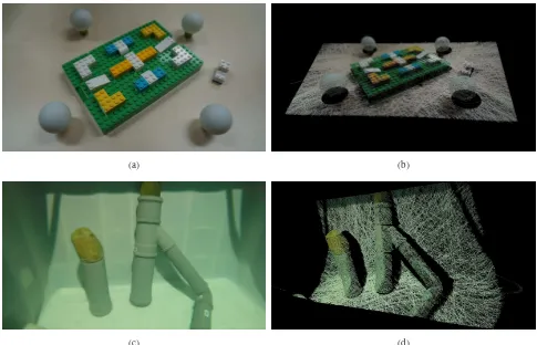
shows a scan of a small scene with LEGO bricks, which is de-picted in Fig. 5(a). Fine details of the bricks can be captured. The underwater scan of the pipe structure in Fig. 5(d) was cap-tured in a water tank shown in Fig. 5(c). For both scans we tried to achieve a baseline in the range of 0.5 m to 1 m. The scan was created using only the automatic white balance of the GoPro camera. Therefore, in the underwater scan the color reproduction is not accurate.
Scans of a chapel and a comparison with LiDAR data created from multiple scans using a Riegl VZ-400 terrestrial laser scan-ner are depicted in Fig. 6. The scan shown in Fig. 6(a) was cap-tured at night. We used flash photography to capture the color information. Measured surfaces in the scene are up to 20 m away from the camera. Hence, we move the cross line laser projector further away from the camera to scan with baselines in the range of 2 m to 3 m. In Fig. 6(b) two scans created using the presented approach are visualized in pink and turquoise. The data was reg-istered with the LiDAR data, which is colored in yellow, using the well known iterative closest point (ICP) algorithm.
Fig. 6(c) shows the point cloud created using the proposed method colored with the point-to-point distance from the point cloud quired using the terrestrial laser scanner. The LiDAR data was ac-quired multiple months before scanning the chapel with the cross line laser system. Therefore, note that the points of the tree in the right part of the image do not match the LiDAR data because the vegetation has changed in the time that passed between the scans. The error histogram is depicted in Fig. 6(d). 78% of the points in the two scans created using the proposed method differ less than 10 cm from the scans captured using the Riegl VZ-400.
5 CONCLUSIONS
This paper presents a line laser scanning system for above-the-water scanning as well as underabove-the-water scanning. We show how self-calibration techniques for line laser scanning by Furukawa and Kawasaki (2009) can be extended to apply to underwater imaging. Moreover, we provide our implementation details to recover robust 3D estimates and show how the geometric con-straints employed in the self-calibration process can also be used to remove outliers, e.g., erroneous detections from reflections in the scene. In first experiments it was demonstrated that good quality scans can be achieved and a similar performance to 3D line laser scanning using online calibration based on known ref-erence planes in the scene is possible. However, further work is necessary to determine the achievable accuracy. For 3D scanning using the proposed method only a single consumer video cam-era and two line laser projectors are necessary, which makes the system very cost efficient.
ACKNOWLEDGMENTS
This work was supported by the European Union’s Horizon 2020 research and innovation programme under grant agreement No 642477 and the DAAD grant “Self-calibrating 3D laser scanner and positioning system for data acquisition in turbid water” under the project ID 57213185.
References
2G Robotics, 2016. ULS-500 underwater laser scan-ner. http://www.2grobotics.com/products/ underwater-laser-scanner-uls-500/. Online, ac-cessed January 20, 2017.
3D at Depth, 2016. SL1 subsea lidar.http://www.3datdepth. com/. Online, accessed January 20, 2017.
Bouguet, J.-Y., Weber, M. and Perona, P., 1999. What do planar shadows tell about scene geometry? In: 1999 IEEE Computer Society Conference on Computer Vision and Pattern Recogni-tion, Vol. 1, IEEE, pp. 1–8.
Br¨auer-Burchardt, C., Heinze, M., Schmidt, I., K¨uhmstedt, P. and Notni, G., 2015. Compact handheld fringe projection based underwater 3D-scanner. The International Archives of Pho-togrammetry, Remote Sensing and Spatial Information Sci-ences40(5), pp. 33–39.
Bruno, F., Bianco, G., Muzzupappa, M., Barone, S. and Razionale, A., 2011. Experimentation of structured light and stereo vision for underwater 3D reconstruction.ISPRS Journal of Photogrammetry and Remote Sensing66(4), pp. 508–518.
Burns, J., Delparte, D., Gates, R. and Takabayashi, M., 2015. Uti-lizing underwater three-dimensional modeling to enhance eco-logical and bioeco-logical studies of coral reefs.The International Archives of Photogrammetry, Remote Sensing and Spatial In-formation Sciences40(5), pp. 61–66.
Dancu, A., Fourgeaud, M., Franjcic, Z. and Avetisyan, R., 2014. Underwater reconstruction using depth sensors. In: SIG-GRAPH Asia 2014 Technical Briefs, ACM, pp. 2:1–2:4.
Digumarti, S. T., Chaurasia, G., Taneja, A., Siegwart, R., Thomas, A. and Beardsley, P., 2016. Underwater 3d cap-ture using a low-cost commercial depth camera. In: 2016 IEEE Winter Conference on Applications of Computer Vision (WACV), IEEE, pp. 1–9.
(a) (b)
(c) (d)
Figure 5: Test scenes and examples of 3D point clouds created using the proposed method.
(a) (b)
0 0.06 0.12 0.18 0.24 0.3
P
o
in
t-to
-p
o
in
t
d
is
ta
n
ce
in
m
(c)
0 0.1 0.2 0.3 0.4 0.5
0 1 2 3
×104
Point-to-point distance in m
N
u
m
b
er
o
f
p
o
in
ts
(d)
Ecker, A., Kutulakos, K. N. and Jepson, A. D., 2007. Shape from planar curves: A linear escape from flatland. In: 2007 IEEE Conference on Computer Vision and Pattern Recogni-tion, IEEE, pp. 1–8.
Eitel, J. U., Vierling, L. A. and Magney, T. S., 2013. A lightweight, low cost autonomously operating terrestrial laser scanner for quantifying and monitoring ecosystem structural dynamics. Agricultural and Forest Meteorology180, pp. 86– 96.
Furukawa, R. and Kawasaki, H., 2006. Self-calibration of multi-ple laser planes for 3d scene reconstruction.In: Third Interna-tional Symposium on 3D Data Processing, Visualization, and Transmission, IEEE, pp. 200–207.
Furukawa, R. and Kawasaki, H., 2009. Laser range scanner based on self-calibration techniques using coplanarities and metric constraints. Computer Vision and Image Understand-ing113(11), pp. 1118–1129.
Furukawa, R., Viet, H. Q. H., Kawasaki, H., Sagawa, R. and Yagi, Y., 2008. One-shot range scanner using coplanarity con-straints. In: 2008 15th IEEE International Conference on Im-age Processing (ICIP), IEEE, pp. 1524–1527.
Imaki, M., Ochimizu, H., Tsuji, H., Kameyama, S., Saito, T., Ishibashi, S. and Yoshida, H., 2017. Underwater three-dimensional imaging laser sensor with 120-deg wide-scanning angle using the combination of a dome lens and coaxial optics. Optical Engineering.
Jokinen, O., 1999. Self-calibration of a light striping system by matching multiple 3-d profile maps. In: Proceedings of the 1999 Second International Conference on 3-D Digital Imaging and Modeling, IEEE, pp. 180–190.
Massot-Campos, M. and Oliver-Codina, G., 2014. Underwater laser-based structured light system for one-shot 3D reconstruc-tion.In: Proceedings of IEEE Sensors 2014, IEEE, pp. 1138– 1141.
Massot-Campos, M. and Oliver-Codina, G., 2015. Optical sen-sors and methods for underwater 3d reconstruction. Sensors 15(12), pp. 31525–31557.
Menna, F., Nocerino, E., Troisi, S. and Remondino, F., 2013. A photogrammetric approach to survey floating and semi-submerged objects. In: SPIE Optical Metrology 2013, Inter-national Society for Optics and Photonics.
Morinaga, H., Baba, H., Visentini-Scarzanella, M., Kawasaki, H., Furukawa, R. and Sagawa, R., 2015. Underwater active oneshot scan with static wave pattern and bundle adjustment. In: Pacific-Rim Symposium on Image and Video Technology, Springer, pp. 404–418.
Olson, E., 2011. Apriltag: A robust and flexible visual fiducial system. In: 2011 IEEE International Conference on Robotics and Automation (ICRA), IEEE, pp. 3400–3407.
Salvi, J., Pages, J. and Batlle, J., 2004. Pattern codification strate-gies in structured light systems. Pattern recognition37(4), pp. 827–849.
Shortis, M., 2015. Calibration techniques for accurate mea-surements by underwater camera systems. Sensors 15(12), pp. 30810–30826.
Steger, C., 1998. An unbiased detector of curvilinear structures. IEEE Transactions on Pattern Analysis and Machine Intelli-gence20(2), pp. 113–125.
T¨ornblom, N., 2010. Underwater 3D surface scanning using structured light. Master’s thesis, Uppsala University.
Van den Heuvel, F. A., 1998. 3D reconstruction from a single im-age using geometric constraints.ISPRS Journal of Photogram-metry and Remote Sensing53(6), pp. 354–368.
Winkelbach, S., Molkenstruck, S. and Wahl, F. M., 2006. Low-cost laser range scanner and fast surface registration approach. In: Joint Pattern Recognition Symposium, Springer, pp. 718– 728.
Zagorchev, L. and Goshtasby, A., 2006. A paintbrush laser range scanner. Computer Vision and Image Understanding101(2), pp. 65–86.