A FULLY AUTOMATED PIPELINE FOR CLASSIFICATION TASKS
WITH AN APPLICATION TO REMOTE SENSING
K. Suzuki a*, M. Claesen b, H. Takeda a, B. De Moor b
a Dept. of R&D, KOKUSAI KOGYO CO.,LTD., 2-24-1 Harumi-cho, Fuchu-shi,Tokyo,183-0057, JAPAN - (kumiko_suzuki, hiroshi1_takeda)@kk-grp.jp
b Dept. of Electrical Engineering, KU Leuven, STADIUS Kasteelpark Arenberg 10, 3001 Leuven, Belgium, - (marc.claesen, bart.demoor)@esat.kuleuven.be
ICWG III/VII
KEY WORDS: Automated Machine Learning, Feature Generation, Classification, Meta-heuristic Hyperparameter Optimization, Particle Swarm Optimization, UC Merced Land Use data set
ABSTRACT:
Nowadays deep learning has been intensively in spotlight owing to its great victories at major competitions, which undeservedly pushed ‘shallow’ machine learning methods, relatively naive/handy algorithms commonly used by industrial engineers, to the background in spite of their facilities such as small requisite amount of time/dataset for training. We, with a practical point of view, utilized shallow learning algorithms to construct a learning pipeline such that operators can utilize machine learning without any special knowledge, expensive computation environment, and a large amount of labelled data. The proposed pipeline automates a whole classification process, namely feature-selection, weighting features and the selection of the most suitable classifier with optimized hyperparameters. The configuration facilitates particle swarm optimization, one of well-known metaheuristic algorithms for the sake of generally fast and fine optimization, which enables us not only to optimize (hyper)parameters but also to determine appropriate features/classifier to the problem, which has conventionally been a priori based on domain knowledge and remained untouched or dealt with naïve algorithms such as grid search. Through experiments with the MNIST and CIFAR-10 datasets, common datasets in computer vision field for character recognition and object recognition problems respectively, our automated learning approach provides high performance considering its simple setting (i.e. non-specialized setting depending on dataset), small amount of training data, and practical learning time. Moreover, compared to deep learning the performance stays robust without almost any modification even with a remote sensing object recognition problem, which in turn indicates that there is a high possibility that our approach contributes to general classification problems.
* Corresponding author
1. INTRODUCTION
In recent years, deep learning has become a prominent class of methods for complex learning tasks including remote sensing (Krizhevsky et al., 2012; Basu et al., 2015). The key advantage of deep learning is that it can automatically learn suitable data representations, principally enabling these methods to surpass the performance of traditional approaches, which in turn requires a lot of labelled data and computational resources to train such flexible models. In contrast, traditional remote sensing approaches combine feature generators that are defined before the machine learning phase with shallow classifiers. Since these approaches essentially impose prior knowledge, they considerably reduce the learning requirements, such as the amount of labelled data and the computation resources, compared to deep learning. However, as a matter of fact, most studies in traditional shallow learning algorithms domain have focused only on learning algorithms or feature generators separately, and fail to jointly optimize the combination, resulting in suboptimal performance.
To facilitate rapid prototyping on novel data sets, we enhanced these traditional learning pipelines by investigating the potential of jointly determining feature generators, their corresponding weights and subsequent classifiers in a fully automated way.
Some researchers have approached this type of automation using Bayesian optimization methods (Martinez-Cantin, 2014; Komer, 2014), which on the other hand require good prior distributions on free hyperparameters, which are difficult to obtain. Therefore, we specifically optimize the generalization performance of a full learning approach using particle swarm optimization (PSO), which is not overly sensitive to its own configuration.
2. PROPOSED METHOD
Two main processes in image recognition, feature extraction and classification, necessitate time-consuming tasks: establishing the model by combining them and tuning parameters of features and hyperparameters of a classifier. In order to realize a configuration such that operators are free from such a special tuning skill, we propose a whole learning pipeline which optimize those tuning phases automatically.
2.1 Automatic Optimization
Automatic (hyper)parameter optimization which optimizes these steps jointly is essential, where technical knowledge and experiments in machine learning are determined by itself. Considering the current state-of-practice: (i) people tend to The International Archives of the Photogrammetry, Remote Sensing and Spatial Information Sciences, Volume XLI-B3, 2016
optimize hyperparameters of classifier while leaving the features untouched and (ii) hyperparameters of classifier are typically optimized using grid search or random search, which perform quite poorly, we automate the joint optimization of learning algorithms and their respective (hyper)parameters by means of a meta-heuristic optimization algorithm, which performs fast and well in general. According to the level of automation, we design three levels of configuration as illustrated in Figure 1. The search space of the configurations consists of three types of parameters: (i) Feature parameters: parameters of feature extraction, (ii) Feature weight: weights over a set of features, and (iii) Classifier parameters: selection of classifier and respective hyperparameters. In the first basic configuration (Config.1), only one defined feature is used for feature extraction at each experiment, for which parameters are set manually by users, while hyperparameters of classifiers are automatically optimized, which includes determining the most suitable classifier. With this configuration, we will discuss how each feature works, how hyperparameters of classifiers are optimized, and how the optimization affects results. In the second configuration (Config.2), all features are concatenated and used as features. The weights over sets of features are optimized in addition to tuning hyperparameters of classifiers, from which we discuss how weighting works and conclude if weighting is effective or not. Finally, in the last configuration (Config.3), we optimize all parameters automatically including feature parameters, which in turn requires users neither to select parameters nor to a good combination of features and classifier.
Figure 2 illustrated a search space associated to the fully optimized configuration (Config.3), where feature parameters, weights of features and hyperparameters of classifiers are automatically optimized given box constraints. At each iteration, one classifier is selected (i.e. using indices likewise a discrete parameter) and only its hyperparameters are optimized. This search space regarding classifiers indicates that a classifier with less hyperparameters is more likely to be selected, since there is a higher probability of detecting the optimal point in a small search space (caused by less hyperparameters) than in a larger one. In other words, the number of hyperparameters implies the speed of convergence. Moreover, the effective range of hyperparameters also plays an important role in selecting classifier.
2.2 Optimization Algorithm
Not only with deep learning, but also with shallow learning algorithms, hyperparameter tuning has been challenging. Practically, hyperparameter tuning has been commonly performed manually or by naive methods such as grid search, which is intuitively understandable but cannot scale up to many dimensions. Aside from naive methods, there are two major
classes of dedicated approaches to tackle this problem: Bayesian optimization and metaheuristic optimization. We eventually select a metaheuristic algorithm, PSO, which is a well-known meta-heuristic optimization algorithm with several useful properties for this task: (i) it can deal with complex objective functions (i.e. the learning pipeline), (ii) is easily parallelizable as each particle can be evaluated independently and (iii) is not overly sensitive to its own configuration. We utilized the Optunity library (Claesen et al., 2014) for implementations.
The main configuration parameters of PSO are the number of particles and the number of generations, which define a trade-off between the probability to find a good solution and
computation time. In our experiments we use 10 particles and 10 generations, resulting in 100 objective function evaluations in total. Candidate solutions are evaluated through 2-fold cross-validation and 10 iterations. Regarding the loss function, we take the area under the receiver operating characteristic curve (AUROC), where ROC curves represent the ratio between the false positive rate and true positive rate at each level of confidence of a classifier.
2.3 Feature Extraction
Feature extraction is a pre-processing phase, which extracts characteristics from input data. We incorporate a several features to the configuration which are handy and commonly used in computer vision domain. Specifically, nine different features are incorporated to the proposed learning pipeline: PCA (principal component analysis) as a baseline, bilateral filter and Gabor filter to emphasize data characteristics, 8-Freeman’s chaincode, Canny edge detector and HOG (histogram of oriented gradients) to enlarge a different view of datasets. Note that 4 different HOG features are incorporated since the HOG
parameters indicates the size of features in images which is difficult to expect beforehand. Given that our goal is to construct a robust configuration, we do not modify these features according to problems. Eventually the parameters to be optimized sum up to 13 as shown in Table 1. In Config.1 and 2, these parameters are fixed manually, and in Config.3 they are optimized automatically. Note that extracted features are normalized between 0 and 1 over training and test data in order to reduce the impact of the absolute range value. Implementations for image processing are based on OpenCV (Bradski, 2000) and scikit-image (Walt et al., 2014).
Figure 1. Three levelled configurations Figure 2. Optimization over a whole learning pipeline
Table 1. The number of parameters of features The International Archives of the Photogrammetry, Remote Sensing and Spatial Information Sciences, Volume XLI-B3, 2016
2.4 Classifiers
By use of extracted features as input data, classification is executed subsequently in the configuration. Specifically, we incorporate three commonly-used classifiers: naive Bayes, random forest, and SVM (linear, polynomial, and RBF kernel), some of which have hyperparameters that operators have to deal with. generate multiple weak models and unify their results to obtain a good prediction (Breiman, 2001). Although there is a profusion of parameters, the main parameters to be adjusted are the number of trees and the number of features used at each split point. With regard to the number of trees, the larger the number of trees the better since we essentially increase samples to take average, consequently reducing the variance by creating many trees, though the improvement is said to even out quickly. Next to that, the larger the estimator the longer it takes to compute so that we set the search space from 10 to 30. As for the number of features used for each split, a suitable value is such that the resulting trees are as uncorrelated to each other as possible. However, there is no rule of thumbs to find this value as it depends on data characteristic. That is, a smaller value is better if each feature is relevant, and a bigger value if each feature is irrelevant. Therefore, to be robust, not specific to the data, we follow the convention, which is the square root of the number of features.
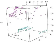
Support vector machine (SVM): a classifier to separate two classes by means of maximizing margin between them (Cortes et el., 1995; Vapnik, 1999). Before the main flow of deep learning, SVM has occupied the domain of computer vision, so that we consider this algorithm as a common handy shallow algorithm, and incorporate it with three kernels: linear kernel, polynomial kernel and RBF kernel. For linear kernel, regularization parameter c is just optimized, resulting in a fast calculation. Linear kernel is essentially used for linearly separable problems though it is said to work well as the number of features increases. As the regularization parameter c increases, the decision boundary can be more complicated to tolerate/avoid classification as well. In addition to regularization parameter, also present in both polynomial and RBF, the degree (for polynomial kernel) and the width of Gaussian function γ (for RBF kernel) should be optimized. As for γ, the smaller the value the more naive the boundary. Note that the optimization of γ is difficult since γ is more sensitive to create the boundary. Next to that, Figure 3 tells us that there is no obvious rule to return the optimal parameters. As such we set the range of c and γ in log scale so as to deal with larger range.
As a whole, the classification problem is defined as a binary problem as SVM can exclusively deal with it. Particularly, we take the one-vs-rest approach since one-vs-one requires making more classifiers therefore resulting in more computation. All implementations about classification are based on scikit-learn (Pedregosa et al., 2011).
3. DEEP LEARNING
Aside from the proposed pipeline, we execute experiments with deep learning to compare the performance. Specifically, we use LeNet network (LeCun et al., 1998), which is known to be a common deep convolutional neural network architecture especially for a handwritten digit recognition. It consists of a convolutional layer followed by a pooling layer, another convolution layer followed by a pooling layer, and then two fully-connected layers. The first convolutional layer computes 32 features for each 5x5 patch, and the second layer has 64 features for each 5x5 patch. The first fully-connected layer with 524 neurons, follows the second fully-connected, and applied to a softmax function. The activation function is the Rectified Linear Unit (ReLU) function. We apply dropout before the readout layer to reduce overfitting. Note that all of these settings follow a Google tensorflow (Abadi et al., 2015) tutorial.
4. DATASETS
Our automated shallow learning approach is targeted for computer vision tasks. Specifically, we focus on a handwritten character recognition problem with the MNIST dataset (LeCun et al., 1998), object recognition problem with the CIFAR-10 dataset (Krizhevsky, 2009), and also object recognition problem with the UC Merced land use dataset (Yang et al., 2010) which is a remote sensing data. As our goal is to construct the learning approach which work with small dataset, we intentionally apply the method to 200 images for test and train each.
MNIST dataset: the MNIST database contains a large volume of handwritten digits (0-9) and was collected from American Census Bureau employees and American high-school students. It contains 10000 examples for training and 50000 examples for testing. Each digit is normalized into a grayscale image and centred in a 28x28 image so that the dimension of data is 784 features (pixels). The previous researchers (Larochelle et al., 2007) built variations of the MNIST basic dataset by imposing various types of noise. To evaluate the model with a different dataset, we utilize one of these noisy versions: the MNIST background images (hereafter the MNIST background). The MNIST background dataset has natural various images as backgrounds. The state of the arts of the MNIST basic goes as low as 0.21% acquired by neural network with dropout in ICML2013 (Wan et al., 2013).
CIFAR-10: the CIFAR-10 dataset contains tiny images belonging to one of 10 categories. The dataset comprises 5000 training images and 1000 test images per class. Each image has 32x32 cells with 3 colour bands. In this paper, we convert these images into grayscale to use this dataset in the same way as the MNIST dataset. Figure 4 illustrates that the CIFAR-10 dataset has distinct characters from the MNIST dataset. Objects that we predict have different shape and size within each category so
Figure 3. Hyperparameters with respect to ROC The International Archives of the Photogrammetry, Remote Sensing and Spatial Information Sciences, Volume XLI-B3, 2016
that characterizing features would be difficult. In fact, the best
result is 96.53% accuracy with fractional max-pooling (Graham, 2014), which is far less compared to the MNIST basic dataset.
UC Merced land use dataset: a remote sensing dataset called UC Merced dataset is tested to confirm robustness of the proposed method. The images were extracted from the USGS National Map Urban Area Imagery collection for various urban areas around the country. The dataset has originally 21 classes and 100 images for each class, from which we draw 10 classes. Although original images are RGB bands and consist of 256x256 pixels, we convert them to grayscale, and resample to 60x60 pixels to adjust the order of input dataset to the MNIST and CIFAR-10 datasets. The main difference between this
dataset and the CIFAR-10 one is that its classes do not always relate to a specific shape, such as agriculture and scrub classes. The current state-of-the-art for this dataset is 94.3% (Negrel et
al., 2014) acquired by aggregating tensor products of local
descriptors.
5. RESULTS
In this chapter, we present our results, through which three levelled optimization configurations are executed successively. Additionally, the results with deep learning are compared to our results to discuss the accuracy and time complexity.
5.1 Configuration. 1
Under Config.1, a classifier is automatically selected with optimal hyperparameters while one feature is manually defined at a feature extraction phase. In order to figure out the characteristics of datasets, feature extractors, and classifiers, we executed several analysis as below.
Feature characteristics: the performance through 10 experiments (e.g. digit 0-9) shown in Figure 5 describes that the MNIST basic dataset returns mostly over 90% AUROC value for each feature except Canny edge detection. Although Canny edge detection normally performs excellent when the edge is clear, handwritten characters in this case sometimes include too thin or light strokes so that edge detection cannot recognize them properly. The performance degrades a lot with the CIFAR-10 dataset. The highest AUROC just records around 75%, showing object recognition in natural image is a more difficult problem. On the other hand, Canny edge detector performs better than with the MNIST datasets where the AUROC is almost 50%. This is because natural images are blurred with bilateral filter well so that Canny edge detector can extract object edges well. Gabor filter and HOG generally return better results than other feature extractors, where four HOGs do not
necessarily perform at the same level since HOG parameters essentially represent the window size, which should correspond to datasets. In case of the UC Merced dataset, the result is highly dispersed within each feature. Indeed, none of the features are effective for all categories, meaning it is difficult to say which feature works well for each category. Hence, selecting an appropriate feature beforehand requires deep insight into the domain.
Regarding the result of cross validation (i.e. the optimal value) and test data, the AUROC value of test data often exceeds the optimal. This is because the amount of training and test data is so small (i.e. 200 images) that the contained data is biased. If we use more training data and the larger number of fold for cross validation, the optimal value should be better.
From left to right over x-axis, features consists of Org (raw data), PCA, Chaincode, Gabor filter, Bilateral filter, Canny edge detector, HOG1, HOG2, HOG3, HOG4. Optimal AUROC is obtained through cross validation, and test data value is calculated with test data. Boxes represent the first and third quartile, a black line inside them is a median value, and plus signs are outliers. Namely, the larger the box is, the more different performance among digits we obtain.
Comparison among classifiers: in Config.1, one classifier is selected eventually through the optimization process. In order to understand how each classifier performs, we evaluated it statistically following the previous work (Demsar, 2006), where Friedman test (Friedman, 1937) and the Nemenyi test (Nemenyi, 1963) are used. Briefly speaking, we compared classifiers head-to-head by means of identifying whether their distance of rank is statically significant. At first, we executed Friedman test of which null hypothesis is all the classifiers are equivalent (i.e. their ranks are equal). Since the p-value was 2.06 e −39 < 0.05, we rejected null hypothesis, meaning at least one classifier has a significantly different rank. Then, we used the Nemenyi
post-From left to right, the MNIST basic, MNIST background, CIFAR-10, UC Merced dataset
Figure 5. Performance by each features with Config. 1 Figure 4. Datasets
hoc test for pairwise comparisons between all classifiers. Critical distance between each classifier is calculated as below:
where the number of approaches k are the number of classifiers (i.e. 5), the number of samples N is the number of experiments which is for each digit for each feature for each of the datasets (i.e. 10 · 9 · 4), and the critical values qα is driven from the Studentized range statistic divided by √2 (≈2.728). If the difference of the average rank between two classifiers is more than critical difference, we can conclude that their performance is statistically different. Note that the difference in this diagram is just a difference of rank so that the effect size (i.e. the difference in ROC curve) cannot be judged here. In other words, the goal here is just to compare the rank of classifiers but not to compare their actual empirical performance. Figure 6 illustrates the rank distance visually, indicating SVM polynomial is the best classifier significantly whereas the difference between all the other classifiers is not significantly different. This result is already different from a general opinion that SVM RBF often works better than SVM polynomial. Hence, selecting the best classifier that works for each dataset/digit properly is not necessarily easy.
Value represents the average rank of the classifier. CD: critical distance, RF: random forest, NB: naive Bayes, SVMR: SVM with RBF kernel, SVMP: SVM with
polynomial kernel, SVML: SVM with linear kernel.
Figure 6: Comparison of classifiers over all MNIST experiments
Classifier Selection: our experiments indicate that SVM polynomial is best, despite SVM RBF being more popular in literature of the computer vision domain. To assess the best possible performance of SVM with RBF kernel, we performed another round of tuning using only SVM-RBF (i.e. c and γ) on a trial basis, by which we attempt to see if the performance of SVM-RBF is indeed less than SVM-polynomial. Figure 7 shows that the results driven with SVM-RBF is the same or less than those with polynomial kernel described in Figure 5. As such, we can conclude that the configuration brings us unexpected better classifier for this problem (i.e. SVM with polynomial kernel).
5.2 Configuration. 2
As shown in the previous section, ’trial and error’ to find an appropriate feature specific to the dataset is cumbersome. Thus, in the second configuration, all 9 features (i.e. PCA, chaincode, Gabor filter, bilateral filter, Canny edge detection, and 4 HOGs) are weighted and used at the same time. Specifically, three types of experiments are executed as variants: (1) All; just
concatenating all features and optimizing hyperparameters of classifiers (i.e. no weighting), (2) All_w; concatenating all features and optimizing weights over a set of features in addition to hyperparameters of classifiers, and (3) All_pca; executing PCA over all filter banks and optimizing hyperparameters of classifiers.
In Figure 8, the results with these three settings are shown, in which the performance is generally better than the previous configuration. The improved performance indicates that the data representations induced by different features carry complementary information which can be exploited by the subsequent classifiers. On the other hand, although the performance with all weighted features is high in general, the difference between the three settings is not so large. In case of
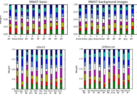
CIFAR-10 and UC Merced datasets, the performance with weighted features is even worse compared to just concatenating features or PCA with concatenated features. This is because the final classifier is mostly random forest or naïve Bayes as shown in Figure 9, which are agnostic to individual feature scales yet the number of parameters to be optimized increases, meaning optimization for weighting eventually is useless for this problem.
X-axis represents digits, under which the selected classifier is noted. NB: naïve Bayes, RF: random forest, linear: SVM linear, poly: polynomial, rbf: RBF
5.3 Configuration. 3
Although the previous section described that concatenating features clearly improves performance, leading to save time to select an appropriate feature, it is still painful for operators that they are required to tune parameters of features manually (e.g. Figure 7. Performance by each feature only with SVM-RBF
The values on x-axis represent median
Figure 8. Performance with Config.2 for each digit/category
Figure 9. Weight value on features for each digit/category The International Archives of the Photogrammetry, Remote Sensing and Spatial Information Sciences, Volume XLI-B3, 2016
the window size of bilateral filter). Therefore, in the configuration 3, we offer a fully optimized configuration, where parameters of features and classifiers are optimized jointly. Note that we just use one HOG feature in this configuration instead of 4 HOG features generated with different parameters since PSO would choose the most appropriate parameters for HOG.
Figure 10 shows that the performance is almost the same as Config.2. That is, the fully optimized configuration provides us the feature parameters comparable to those brought by human beings. On the other hand, there are more parameters to optimize in the full optimization, resulting in more runtime.
5.4 Deep Learning
So far we have reported that our fully automated pipeline brought a good performance with shallow algorithms over small datasets. Given the fact that deep learning algorithms, known to work well with big data, have been in spotlight these days, we applied them to the same small datasets, composed of 200 images each, for comparison. As shown in Table 2, the performance is far lower than the one with Config.2 and 3, meaning a basic deep learning network is not capable of compensating the lack of prior knowledge with a small dataset. Additionally, given the network architecture is designed to the MNIST basic initially, we can conclude that the deep learning network architecture is specific to the dataset while our approach is robust.
5.5 Time Complexity
Practically speaking, time complexity is a big concern as well as performance and the required size of sample. Table 3 shows that all algorithms except Config.3 run in a realistic time. Config.3 is the equivalent of deep learning in a sense that it requires no prior knowledge for feature extraction and classifiers, resulting in extraordinary runtime. As such, our pipeline provides two different levelled configurations according to user’s demand. That is, in Config.2, users can save time to run optimization but still have to tune feature parameters themselves and in Config.3 users do not select parameters for features, but need more time to run. Next to that, depending on the priority, we can save time by removing random forest or Gabor filter which mainly takes time to calculate.
CONCLUSION
We proposed a whole learning pipeline where shallow classifiers and feature extraction are optimized jointly by Particle Swarm Optimization algorithm. The proposed method acquired high performance over four small different datasets, showing that the pipeline performs well (1) over different kinds of datasets, with (2) no specific tuning experience/domain knowledge, (3) small amount of labelled data, and (4) cheap hardware, all of which exceeds the prerequisites of deep learning algorithms. Additionally, the characteristic that we can incorporate another features to the configuration would also extend our approach to different fields. Taking an example, we
can even incorporate the filter banks driven by deep learning. On the other hand, classification of cifar-10 and remote sensing dataset have not achieved the performance up to a practical usage mostly because of their various shape and texture. We can improve them simply by using 3 bands instead of a grey scale. Moreover, discussion about features which deal with rotated images such as SIFT is left for the future work.
ACKNOWLEDGEMENTS
STADIUS members are supported by Flemish Government: FWO: projects: G.0871.12N (Neural circuits), IWT: TBM Logic Insulin (100793), TBM Rectal Cancer (100783), TBM IETA (130256); PhD grant #111065, Industrial Research fund (IOF): IOF Fellowship 13-0260; iMinds Medical Information Technologies SBO 2015, ICON projects (MSIpad, MyHealthData) VLK Stichting E. van der Schueren: rectal cancer; Federal Government: FOD: Cancer Plan 2012-2015 KPC-29-023 (prostate); COST: Action: BM1104: Mass Spectrometry Imaging.
REFERENCES
Abadi, M., et al., and Zheng, X., 2015. TensorFlow: Large-scale machine learning on heterogeneous systems, Software available from tensorflow.org.
Basu, S., Ganguly, D., Mukhopadhyay, S., DiBiano, R., Karki, M., and Nemani, R., 2015. DeepSat - A Learning framework for Satellite Imagery. CoRR abs/1509.03602.
Table 3. Median of running time (sec/hour) per digit/category of the proposed methods and deep learning
Claesen, M.,Simm, J., Popovic, D., Moreau, Y., and De Moor, B., 2014. Easy hyperparameter search using Optunity. arXiv preprint arXiv:1412.1114.
Demsar, J., 2006. Statistical comparisons of classifiers over multiple data sets. J. Mach. Learn. Res., 7:1–30.
Friedman, M., 1937. The use of ranks to avoid the assumption of normality implicit in the analysis of variance.
j-J-AM-STAT-ASSOC, 32(200):675–701.
Graham, B., 2014. Fractional Max-Pooling, CoRR, 1412.6071.
Komer, B., Bergstra, J., and Eliasmith, C., 2014. Hyperopt-sklearn: Automatic hyperparameter configuration for scikit-learn. In ICML 2014 AutoML Workshop, pp. 8.
Krizhevsky, A., 2009. Learning multiple layers of features from tiny images. Technical report, Computer Science Department, University of Toronto.
Larochelle, H., Erhan, D., Courville, A., Bergstra, J., and Bengio, Y., 2007. An empirical evaluation of deep architectures on problems with many factors of variation. In Proceedings of
the 24th International Conference on Machine Learning (ICML), pp.473–480
LeCun, Y., Bottou, L., Bengio, Y., and Haner, P., 1998. Gradient-based learning applied to document recognition. In Proceedings of the IEEE, pp. 2278-2324.
Martinez-Cantin, R., 2014. Bayesopt: A bayesian optimization library for nonlinear optimization, experimental design and bandits. Journal of Machine Learning Research, Vol.15, pp. 3735-3739.
Mnih, V., and Hinton, G., 2010. Learning to detect roads in high-resolution aerial images. In Proceedings of the 11th
European Conference on Computer Vision (ECCV), pp.
210-223.
Negrel R., Picard, D., and Gosselin, P., 2014. Evaluation of second-order visual features for land-use classification. In 12th International Workshop on Content-Based Multimedia Indexing,
Nemenyi, P., 1963. Distribution-free multiple comparisons. Technical report, Princeton University
Pedregosa, F., et al., 2011. Scikit-learn: Machine learning in Python. Journal of Machine Learning Research, pp. 2825–2830.
Vapnik, V., 1999. An overview of statistical learning theory. Trans. Neural Network, pp.988–999.
Walt, S., et al., 2014. scikit-image: image processing in Python.
PeerJ, 2:e453.
Wan, L., Zeiler, M., Zhang, S., LeCun, Y., and Fergus, R., 2013. Regularization of neural networks using dropconnect. In
Proceedings of the 30th International Conference on Machine
Learning (ICML 2013), pp. 1058–1066.
Yang,Y., and Newsam, S., 2010. Bag-of-visual-words and spatial extensions for land-use classification. In Proceedings of
the 18th SIGSPA-TIAL International Conference on Advances in Geographic Information Systems, pp. 270-279.