A SEMI-RIGOROUS SENSOR MODEL FOR PRECISION GEOMETRIC
PROCESSING OF MINI-RF BISTATIC RADAR IMAGES OF THE MOON
R. L. Kirk1*, J. M. Barrett1, D. E. Wahl2, I. Erteza2, C. V. Jackowatz2, D. A. Yocky2, S. Turner3, D. B. J. Bussey3, G. W. Paterson3
1Astrogeology Science Center, U.S. Geological Survey, 2255 N. Gemini Dr., Flagstaff AZ 86001 ([email protected]) 2
Sandia National Laboratories, Albuquerque, NM 87185
3The Johns Hopkins University Applied Physics Laboratory, Laurel, MD 20723
C o m m issio n IV , W G IV /8
K E Y W O R D S : SAR, bistatic, sensor models, extraterrestrial, Moon
A B S T R A C T :
The spaceborne synthetic aperture radar (SAR) instruments known as Mini-RF were designed to image shadowed areas of the lunar poles and assay the presence of ice deposits by quantitative polarimetry. We have developed radargrammetric processing techniques to enhance the value of these observations by removing spacecraft ephemeris errors and distortions caused by topographic parallax so the polarimetry can be compared with other data sets. Here we report on the extension of this capability from monostatic imaging (signal transmitted and received on the same spacecraft) to bistatic (transmission from Earth and reception on the spacecraft) which provides a unique opportunity to measure radar scattering at nonzero phase angles. In either case our radargrammetric sensor models first reconstruct the observed range and Doppler frequency from recorded image coordinates, then determine the ground location with a corrected trajectory on a more detailed topographic surface. The essential difference for bistatic radar is that range and Doppler shift depend on the transmitter as well as receiver trajectory. Incidental differences include the preparation of the images in a different (map projected) coordinate system and use of “squint” (i.e., imaging at nonzero rather than zero Doppler shift) to achieve the desired phase angle. Our approach to the problem is to reconstruct the time-of-observation, range, and Doppler shift of the image pixel by pixel in terms of rigorous geometric optics, then fit these functions with low-order polynomials accurate to a small fraction of a pixel. Range and Doppler estimated by using these polynomials can then be georeferenced rigorously on a new surface with an updated trajectory. This “semi-rigorous” approach (based on rigorous physics but involving fitting functions) speeds the calculation and avoids the need to manage both the original and adjusted trajectory data. We demonstrate the improvement in registration of the bistatic images for Cabeus crater, where the LCROSS spacecraft impacted in 2009, and describe plans to precision-register the entire Mini-RF bistatic data collection.
* Corresponding author
1 . IN T R O D U C T IO N
This paper is the culmination of a series of publications (Kirk et al., 2010; 2011; 2012; 2013) describing our development of techniques for radargrammetry (analogous to photogrammetry but taking account of the principles by which radar images are formed) and their application to mapping the Moon with Mini-RF images. Our overall goals are to use radar stereopairs to produce digital topographic models (DTMs) of medium resolution and broad coverage, and to control and orthorectify (project onto an existing DTM) images to produce image maps and mosaics with greatly improved positional accuracy.
Here, we describe our approach to processing bistatic observations, in which a signal transmitted from Earth is received on board the spacecraft (Patterson et al., 2016). These observations are of tremendous scientific interest as part of the overall Mini-RF program of searching for ice deposits at the lunar poles (Kirk et al., 2014; Spudis et al., 2009) because the variation of signal strength with the phase angle between transmitter and receiver may distinguish between coherent backscatter in ice (Hapke and Blewett, 1991) and diffuse scattering by blocky surfaces (Nelson et al., 2000). By controlling and rectifying these observations we enable the quantitative analysis of radar-scattering properties on a point-by-point basis with the more extensive monostatic radar images and other remote sensing data such as optical and thermal images and altimetry on a pixel-by-pixel basis.
2 . S O U R C E D A T A
NASA’s Mini-RF investigation consists of two synthetic aperture radar (SAR) imagers for lunar remote sensing: the “Forerunner” Mini-SAR on ISRO’s Chandrayaan-1 (Spudis et al., 2009), and the Mini-RF on the NASA Lunar Reconnaissance Orbiter (LRO) (Nozette et al., 2010), which carried out monostatic observations from 2009 until its transmitter failed in December 2010. After this, the bistatic observations analysed here were obtained by LRO receiving S-band (12.6 cm wavelength) signals transmitted from the Arecibo Observatory (Patterson et al., 2016). Several tens of bistatic observations have been obtained to date, covering both polar and (as a baseline for possible detection of polar ice) nonpolar targets.
projection used for monostatic Level 2 products. The result is very similar visually, but latitude-longitude coordinates can now be calculated by a simple set of map projection equations (Reid, 2010), vastly simplifying the subsequent analysis.
3 . T E C H N IC A L A P P R O A C H A N D M E T H O D O L O G Y
The monostatic and bistatic radar images described above all contain positional offsets caused by errors in the spacecraft trajectory used in processing, plus parallax caused by topography (Fig. 1). Our goal is to correct these errors and distortions. The essential tool is a sensor model: a mathematical and software model capable of computing ground coordinates for a given image line-sample and vice versa. In practice, the model can be divided into two steps: (a) inverting the initial processing to recover the fundamental radar observables (range, and Doppler shift at a specified time) for an image pixel, and (b) determining where a feature with this range and Doppler shift should be located. The opportunity to achieve precision georeferencing comes in the second step, where we can solve for an improved estimate of the spacecraft trajectory that brings the image into best registration with neighboring images and base data such as LOLA altimetry (Smith et al., 2010), i.e., geodetic control, and project the data onto a detailed topographic model of the target (orthorectification). Our bistatic sensor model is implemented in the USGS ISIS system (Anderson et al., 2004) and uses a version of the ISIS bundle adjustment program jigsaw (Edmundson et al., 2012) for the control calculation. The resulting workflow for precision products is analogous to that for monostatic Mini-RF images (Kirk et al., 2013). The devil, as ever, is in the details.
F ig u re 1 . Overlay of LRO Mini-RF bistatic image of Cabeus crater (center) and environs on a mosaic of east-looking monostatic images. Circles show the misalignment of corresponding craters by several km between the uncontrolled east-looking (blue), west-looking (green) and bistatic (red) data products. Polar Stereographic projection, South Pole at bottom,
330° E longitude toward top, grid spacing 5° (lat) by 15° (lon). Box shows the location of Fig. 3.
4 . M O N O S T A T IC V S B IS T A T IC
The two types of radar observations are defined by their geometry. In both cases, the observed quantities are the range to a surface point and its Doppler shift (which is proportional to the time derivative of range) at given point. The difference is that for monostatic radar the transmitter and receiver are at the same location and range thus refers to distance from this point; the points with the same range lie on a sphere centered on the spacecraft (Fig. 2a). For bistatic observations, range is the total distance from transmitter to ground to receiver, and a given range thus defines an ellipsoid with transmitter and receiver at the foci (Fig. 2b). The Doppler shift is proportional to the derivative of the range and is modified accordingly.
F ig u re 2 a . Cartoon illustrating the geometry of monostatic radar imaging. Features are located in terms of their range from the spacecraft and Doppler shift at the time of observation. Range (blue sphere and Doppler (green cone) surfaces intersect in a circle (red). This intersects the planetary surface at two points, only one of which is illuminated. As discussed in the text, monostatic radar images are typically obtained by viewing perpendicular to the trajectory (near zero Doppler shift) rather than “squinted” as shown here.
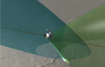
F ig u re 2 b . Geometry of bistatic radar observation. “Range” is the total distance from transmitter (on Earth) to ground to spacecraft so defines an elongated ellipsoid (blue). Doppler shift involves both transmitter and receiver motion but still defines a cone (green).
Mathematically, the location of a ground point x on three intersecting surfaces (Doppler cone, range locus, and planetary surface respectively) can be described as follows:
−2 λρ=−
2 λ
x s−
x
x s−
xi
v=Δf or (1a)
−1
λρ=−
1
λ
x s−
x
x s−
x+ˆ e
⎛
⎝
⎜⎜ ⎞
⎠
where Equations (1a) and (2a) refer to the monostatic case illustrated in Fig. 2a and (1b) and (2b) to the bistatic case in Fig. 2b. In these equations xs is the spacecraft position and v its body-fixed velocity, ˆe is a unit vector pointing to the distant transmitter on Earth, ρ is range, Δf is Doppler shift, λ is the radar wavelength, and R is the planetary radius (or the local radius at the solution point if a topographic model is being used. Though physically fundamental, these differences do not greatly change the operation of the sensor model. In either case, ρ and Δf are readily computed at given time t (which determines xs and v). To compute x given ρ and Δf, it is useful to establish an in-track cross-track radial (ICR) coordinate system centered at xs . Then the in-track and radial components of x are readily eliminated from equations (1)-(3) yielding a single equation for the cross-track component. In the monostatic case, this equation is quadratic and is readily solved analytically (with the choice of sign between the two roots corresponding physically to left-looking or right-left-looking observation). In the bistatic case a quartic equation is obtained, and it is more convenient to find the solution by numerical means.
The formatting of the image data turn out to have a much larger impact on the sensor model design. For the Mini-RF monostatic observations, each Level 1 image line represents an equal increment in time and contains those features that were observed at zero Doppler shift (i.e., at minimum range, or directly to the side of the spacecraft) at that time. The image labels contain the coefficients of polynomials that can be used to convert sample number to range. Our initial model of the geometry of the bistatic observations (Kirk et al., 2014) went astray by following this monostatic example too closely.
The key consideration for modeling the bistatic observations turns out to be that they are obtained at nonzero squint angle, i.e., with the radar antenna aimed ahead or behind rather than directly to the side of the spacecraft trajectory. Squinting is equally possible for monostatic radar observations but is seldom used in practice, so that most often Δf = 0 in Eq. (1a) and this provides a simple means to determine the time at which a point is observed. For Mini-RF bistatic observations, squinting is essential to observing targets of geologic interest (polar craters and their low-latitude analogues) at specific phase angles. Modeling the squint is critical to precision geometric processing because topographic parallax always occurs along the line between a surface feature and the location of the radar when it was observed. For (unsquinted) bistatic images this is perpendicular to the flight track, but for squinted images parallax distortions are diagonal.
5 . A S E M I-R IG O R O U S S E N S O R M O D E L
The simplest conceptual approach to a radar sensor model would be to use the trajectory and surface models that were used in making the original image to back-calculate the time, range, and Doppler shift at which a pixel was observed, and then use an updated trajectory and better topographic model to project the pixel onto the ground in a more accurate location. Unfortunately, the ISIS system is not designed to facilitate this kind of “double bookkeeping” of trajectory or surface models. We therefore divide our analysis of Mini-RF bistatic images into a preprocessing phase, in which we fit polynomial models to key variables (time, range, and Doppler shift) calculated from the original trajectory, followed by a processing phase in which
we use these fits to approximate the observables and then rigorously compute surface coordinates based on an updated trajectory and detailed surface. This approach is a practical hybrid between rigorous (physics-based) and non-rigorous (based purely on approximating functions) sensor models.
5 .1 P re p ro c e ssin g
This phase begins with calculation of the time at which each pixel is closest to the antenna boresight axis, as defined by the trajectory and pointing history of the spacecraft that were used to form the image and the latitude, longitude, and (assumed zero) elevation of the pixel. The time is the average of the (relatively short) period over which a given ground feature is observed, and the spacecraft position defines the direction in which parallax distortions operate. Next, we calculate the range and Doppler shift for each pixel at its time of observation, still based on the nominal trajectory. We then fit polynomials to represent observation time as a function of image sample and line, range as a function of sample and time, and Doppler shift as a function of sample and time. In the ideal case of flight at constant height over a planar surface, time, sample, and line would be linearly related and the equations relating range and Doppler shift to sample would be time-independent. The curvature of the Moon and the slight variation in height of the spacecraft’s elliptical orbit create the need for higher order correction terms. Guided by examining the residuals to our polynomial fits for a typical image described in the next section, we arrived at the following representations:
t = t00 + ts s + tss s2 + tl l, (4) practice are normalized to the interval -1 to 1 when used as the independent variables in these polynomials to minimize roundoff errors), Δf is Doppler shift, and the subscripted quantities are the polynomial coefficients. The polynomial in Eq. (7) is convenient for the inverse calculation of image coordinates for a ground point, but note that Eq. (4) is linear in l so a separate polynomial is not needed to compute l from s and t. The final step of preprocessing is to store the polynomial coefficients in the image labels and remove the map projection information (which was crucial to establishing them) so that ISIS henceforth treats the image as a Level 1 (image with known sensor model) rather than Level 2 (map projected) product.
5 .2 R a d a rg ra m m e tric P ro c e ssin g
Doppler shift at the same line and sample. To make the control adjustment by jigsaw possible, we also provide the means to calculate range and Doppler errors for a ground point at fixed time and the partial derivatives of these errors with respect to the spacecraft position and velocity.
6 . V A L ID A T IO N : C A B E U S C R A T E R
To test our sensor model, we selected a fairly typical high-latitude bistatic observation covering part of Cabeus crater, site of the 2009 impact of the LCROSS spaceeraft (Colaprete et al., 2010). Known informally as 2013-346 (the day of acquisition, 12 December 2013) and formally as LST_20279_1S1_ XIU_80S79_V1, this image is centered near 79.3°E, 80.9°S (Patterson et al., 2016). Phase angles range from 0.1° to 28°. Because of the evolving state of the bistatic data products, the data and metadata for testing had to be collected from a variety of sources: PDS labels for the original (not map projected) image for most quantities, map-projected image and projection parameters from Sandia, and a time-of-observation map generated at APL. The first stage of testing was to determine the appropriate order to use for the polynomial models as reflected in Eq. (4) to (7). We found empirically that for the order of polynomials given here, the maximum error in the fit for t over the image was 0.1 s, corresponding to about 0.02 of the total integration time (set by the beamwidth) during which a point is observed. The root mean square (RMS) in r was 9 m or about 0.03 pixel, that in Δf was 0.h Hz equivalent to 0.04 pixel, and that for s was 0.01 pixel. The RMS error of closure, calculating from s to t by (4) and back to s by (7) was less than 0.01 pixel. This is adequate for stereoanalysis (typical stereomatching errors are ≥0.2 pixel) and more than adequate for georeferencing of the data for purposes of cross-comparison.
The errors in our polynomial approximations are also much smaller than the positional errors of the source data and their supporting metadata. During the production of controlled monostatic mosaics of the lunar north pole (Kirk et al., 2013) we discovered that along-track adjustments often exceeding a kilometer were required to bring the east- and west-looking image sets into alignment with one another and with ground truth provided by LOLA. Similar offsets are seen in the south polar data sets before control, as is visible in Fig. 1. During the process of making controlled south polar mosaics, we discovered that these errors can be attributed to systematic inaccuracy in the start times recorded for the individual images. For the polar monoscopic data sets (July 2009 to July 2010) timing errors increase linearly from zero to between 1.0 and 1.3 second and then reset to zero repeatedly over the course of the mission. The cause of the errors is not presently understood, but correcting start times with a piecewise-linear function of orbit number reduced the mismatch between image sets from ~3 km to ~30 m, greatly simplifying the process of collecting tiepoints to produce controlled mosaics for the south pole. The offset between the Cabeus bistatic observation and the LOLA base is about 2.7 km, indicating a timing error on the order of 1.6 s, slightly larger than the maximum error in the monostatic image sets. Unfortunately, the bistatic observation was obtained so long after the monostatic mosaic sequences that it is impossible to determine whether the repeating pattern of timing errors persisted. Because the typical positional error after time correction (~30 m) is smaller than the pixel scale of the bistatic observation (100 m) we did not attempt to further refine the georeferencing by bundle adjustment with jigsaw. Figure 3 shows the excellent alignment of the bistatic data with the controlled monostatic image mosaics after applying a start time
correction. There is no evidence of misregistration of small albedo or topographic features at 100 m/pixel scale.
F ig u re 3 . Comparison of time-corrected and orthorectified bistatic image of the lunar south polar region (blue) with east-looking (green) and west-east-looking (red) controlled mosaics of monostatic images for the region outlined in Fig. 1. Projection is the same as in Fig. 1 with north approximately at top.
7 . O N G O IN G W O R K
Our ultimate goal is to georeference and orthorectify all of the Mini-RF bistatic images so that they can be compared directly with monostatic radar observations and with other data sets such as topography, temperature, and hydrogen abundance. For this to be practical, the necessary metadata must be organized more systematically than they were at the time of this study. The first step toward this goal has been to re-deliver the bistatic observations to the PDS in map-projected form and with mapping parameters included in the labels. The time-of-observation map, which is crucial to enabling our semi-rigorous sensor model, is not accommodated in the PDS file design so it will be supplied as an ancillary data product. We are currently working to reorganize the ISIS software from its initial research form described above to a practical implementation that will make use of the updated PDS labels and data products. This software will be publically released (at http://isis.astro-geology.usgs.gov). We also plan to test whether the timing correction is adequate to georeference all the bistatic observations or whether geodetic control with jigsaw can significantly improve the results.
R E F E R E N C E S
Anderson J. A. et al., 2004. Modernization of the Integrated Software for Imagers and Spectrometers. Lunar Planet. Sci. XXXV, 2039.
Colaprete, A., et al., 2010. 2010. Detection of Water in the LCROSS Ejecta Plume. Science 330, 6003, 463.
Hapke B. and Blewett, 1991. Coherent backscatter model for the unusual radar reflectivity of icy satellites. Nature 352, 46.
Kirk R. L. et al., 2010. Radargrammetry with Chandrayaan-1 and LRO Mini-RF images of the Moon: Controlled mosaics and digital topographic models. Lunar Planet. Sci. XLI, 2428.
Kirk R. L., et al., 2011. Next steps in radargrammetry of the Moon: Targeted stereo observations and controlled mosaic production. Lunar Planet. Sci. XLII, 2392.
Kirk R. L., et al., 2012. Progress in radargrammetric analysis of Mini-RF lunar images. Lunar Planet. Sci.XLIII, 2772.
Kirk R. L. et al., 2013. A radargrammetric control network and controlled Mini-RF mosaics of the Moon’s north pole…at last! Lunar Planet. Sci.. XLIV, 2920.
Kirk, R.L., et al., 2014. Precision geometric processing of Mini-RF bistatic radar images of the Moon. Lunar Planet. Sci. XLV, 2548.
Nozette S. et al., 2010. The Lunar Reconnaissance Orbiter Miniature Radio Frequency (Mini-RF) Technology Demonstration. Space Sci Rev, 150, 285.
Nelson R. M. et al., 2000. The Opposition Effect in Simulated Planetary Regoliths. Reflectance and Circular Polarization Ratio Change at Small Phase Angle. Icarus 147, 545.
Patterson, G. W., et al. 2016 Bistatic radar observations of the Moon using Mini-RF on LRO and the Arecibo Observatory. Icarus, in press.
Reid M., 2010. PDS Data Product SIS for Mini-RF, MRF-4009, February 25 2010.
Smith D. E. et al., 2010. The Lunar Orbiter Laser Altimeter Investigation on the Lunar Reconnaissance Orbiter Mission. Space Sci. Rev. 150, 209.
Spudis P. D. et al., 2009. Mini-SAR: An imaging radar experiment for the Chandrayaan-1 mission to the Moon. Curr. Sci. (India) 96, 533.