q
An earlier version of this paper appeared under a slightly di!erent title as ORC Working Paper OR 256-91.
*Corresponding author. Tel.: 10-408-2576; fax: 10-408-9162. E-mail address:[email protected] (A.P.M. Wagelmans)
Parametric analysis of setup cost in the economic lot-sizing
model without speculative motives
qC.P.M. Van Hoesel
!
, A.P.M. Wagelmans
",
*
!Department of Quantitative Economics, Maastricht University, P.O. Box 616, NL-6200 MD, Maastricht, Netherlands
"Econometric Institute, Erasmus University Rotterdam, P.O. Box 1738, 3000 DR Rotterdam, Netherlands Received 12 January 1999; accepted 27 May 1999
Abstract
In this paper we consider the important special case of the economic lot-sizing problem in which there are no speculative motives to hold inventory. We analyze the e!ects of varying all setup costs by the same amount. This is equivalent to studying the set of optimal production periods when the number of such periods changes. We show that this optimal set changes in a very structured way. This fact is interesting in itself and can be used to develop faster algorithms for such problems as the computation of the stability region and the determination of all e$cient solutions of a lot-sizing problem. Furthermore, we generalize two related convexity results which have appeared in the literature. ( 2000 Elsevier Science B.V. All rights reserved.
Keywords: Economic lot-sizing; Parametric analysis; Stability; E$cient solutions; Dynamic programming
1. Introduction
In 1958 Wagner and Whitin published their
seminal paper on the `Dynamic Version of the
Economic Lot-Size Modela, in which they showed
how to solve the problem considered by a dynamic programming algorithm. It is well known that the same approach also solves a slightly more general problem to which we will refer as the economic lot-sizing problem (ELS). Recently, considerable improvements have been made with respect to the complexity of solving ELS and some of its
special cases (see [1}3]). Similar improvements
can also be made for many extensions of ELS (see [4]).
In this paper we consider the important special case of ELS in which there are no speculative mo-tives to hold inventory, i.e., the marginal cost of producing one unit in some period plus the cost of holding it until some future period is at least the marginal production cost in the latter period. For
this model we analyze the e!ects of varying all
setup costs by the same amount. This is equivalent to studying the set of optimal production periods when the number of such periods changes. We will show that this optimal set changes in a very struc-tured way. This fact is interesting in itself and can be used to develop faster algorithms for such prob-lems as the computation of the stability region and
the determination of all e$cient solutions of a
lot-sizing problem. Furthermore, we will generalize
two related convexity results which have appeared in the literature.
The paper is organized as follows. In Section 2 we state several useful results about the economic lot-sizing problem without speculative motives. In Section 3 we perform a parametric analysis of the problem. We will characterize how the optimal solution changes when all setup costs are reduced by the same amount and we will present a linear time algorithm to calculate the minimal reduction for which the change actually occurs. In Section 4 we discuss applications of the results of Section 3. Finally, Section 5 contains some concluding remarks.
2. The economic lot-sizing problem without specu-lative motives
In the economic lot-sizing problem (ELS) one is
asked to satisfy at minimum cost the known
de-mands for a speci"c commodity in a number of
consecutive periods (theplanning horizon). It is
pos-sible to store units of the commodity to satisfy future demands, but backlogging is not allowed. For every period the production costs consist of two components: a cost per unit produced
and a "xed setup cost that is incurred whenever
production occurs in the period. In addition to the production costs there are holding costs which are linear in the inventory level at the end of the period. Both the inventory at the beginning and at the end of the planning horizon are assumed to be zero.
We will use the following notation:
¹: the length of the planning horizon,
d
Furthermore, we de"ned
ij,+jt/idt for alli,jwith
1)i)j)¹.
As shown in [3] an equivalent problem results when all unit holding costs are taken 0, and for all
i3M1,2,¹Nthe unit production costp
This reformulation can be carried out in linear time and it changes the objective function value of all feasible solutions by the same amount. From now on we will focus on the reformulated problem.
In this paper, we assume that c
i*ci`1 for all
i3M1,2,¹!1N. Note that if ci were less than
c
jfor somej'i, then this could be perceived as an
incentive to hold inventory at the end of periodi(in
order to avoid that the higher unit production cost
in periodjwill have to be paid). Under our
assump-tion on the unit producassump-tion costs this incentive is not present. Therefore, this special case is known as theeconomic lot-sizing problem without speculative
motives. Note that in the model originally
con-sidered by Wagner and Whitin [5] it is assumed
thath
i*0 andpi"0 for alli3M1,2,¹N. Because
c
i"pi#+Tt/iht, it is easily seen that this model is
an example of a lot-sizing problem without specu-lative motives.
It is well known that economic lot-sizing prob-lems can be solved using dynamic programming. For problems without speculative motives, the dy-namic programming algorithm can be implemented
such that it requires only O(¹) time (see [1}3]). We
will now brie#y review such an implementation.
The key observation to obtain a dynamic
pro-gramming formulation is that it su$ces to consider
only feasible solutions that have thezero-inventory
property, i.e., solutions in which the inventory at the beginning of production periods is zero. The latter
implies that if i andj are consecutive production
periods with i(j, then the amount produced in
periodi equals d
ij~1. From now on, we will only
consider solutions with this property. Also, note that we may assume that setups only take place in production periods, even if some of the setup costs are zero. Hence, solutions can completely be de-scribed by their production periods which coincide with the periods in which the setups occur.
Let the variable F(i), i3M1,2,¹N, denote the
value of the optimal production plan for the in-stance of ELS with the planning horizon truncated
after periodi, and de"neF(0),0. Fori"1,2,¹
the value ofF(i) can be calculated using the
follow-ing forward recursion:
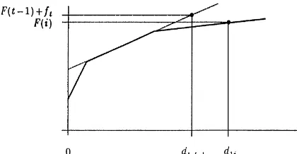
F(i):"min
0:txi
MF(t!1)#f
Fig. 1. Determination ofF(i).
t) and draw the line with slope ct that passes
through this point. It is easy to verify that F(i) is
equal to the value of the concave lower envelope of
these lines in coordinated
1ion the horizontal axis.
After constructing the line with slopec
i that passes
through (d
1i,F(i)#fi`1), we update the lower
en-velope and continue with the determination of
F(i#1).
The running time of this algorithm depends on the complexity of evaluating the lower envelope in certain points on the horizontal axis and the com-plexity of updating the concave lower envelope. Because lines are added in order of non-increasing
slope, the total computational e!ort for updating
the lower envelope (i.e., over all¹iterations) can be
done in linear time. (We use a stack to store the breakpoints and corresponding line segments of the lower envelope.) The fact that the points in which the envelope is evaluated have a non-de-creasing horizontal coordinate can be used to
es-tablish an O(¹) bound on the total number of
operations required for those evaluations. Hence, the algorithm runs in linear time.
For convenience we will assume from this point
on thatd
1'0. Hence, period 1 is the"rst
produc-tion period in every feasible solution. Let
i3M2,2,¹N, then h3M1,2,i!1N is called an
optimal predecessor ofi if periodhis the last
pro-duction period beforeiin some optimal solution in
whichiis a production period. This means thathis
such that F(i!1)"MF(h!1)#f
h#chdh,i~1N.
Periodhis referred to as an optimal predecessor of
¹#1 if it is the last production period in some
optimal solution.
The following result is a slight generalization of the well-known planning horizon theorem due to Wagner and Whitin. It will be used frequently later on.
Lemma 1. Let 1)h(i(j(k)¹#1 be such that h is an optimal predecessor of k and i is an optimal predecessor of j,then both h and i are optimal predecessors of both j and k.
Proof. We know that
F(j!1)"F(i!1)#f
Combining these inequalities leads to
c
hdj,k~1)cidj,k~1.
It is easily seen that the lemma holds ifd
j,k~1"0.
Assuming d
j,k~1'0, we obtain ch)ci. Because
h(i we already know that c
h*ci. Therefore, it
must hold that c
h"ci. Substituting this into (1)
Hence, equality must hold in both (1) and (2), which
implies the desired result. h
In the next section we perform a parametric analysis of the setup costs of the economic lot-sizing problem without speculative motives.
3. Parametric analysis
In this section we study the parametric problem
with setup costs of the form f
i!j, i"1,2,¹.
Here allf
Fig. 2. Structure of optimal solution in Theorem 1.
the domain of the parameterjis the interval [0,K],
whereK)min
i/1,2,TMfiN. The main issue we will
deal with is the following. Suppose we are given an optimal solution for the lot-sizing problem for
j"0. Assume that the set of production periods
is Mi
1,2,iqN, where 1"i1(i2(2(iq and
q(¹; also de"ne i
q`1,¹#1. When j is
in-creased, solutions with more thanqsetups become
relatively more attractive (and solutions with less
than q setups become less attractive). We would
like to determine the smallest value ofj3[0, K], if
any, such that there exists an optimal solution with
at least q#1 setups. Furthermore, we are also
interested in that optimal solution itself.
Letj@denote the parameter value we are looking
for. We will use an approach to "nd this value
which is based on a natural decomposition
of the problem. To this end we de"ne ELS(t),
t3M2,2,q#1N, as the parametric lot-sizing
prob-lem with planning horizon consisting of the
"rst i
t!1 periods. Furthermore, we let jt,
t3M2,2,q#1N, denote the smallest value in
[0, K] for which there exist an optimal solution for
ELS(t) with at leasttsetups;j
tis de"ned to beRif
there does not exist such a solution for any
j3[0, K]. Clearly,j@exists and is equal to j
q`1 if
and only if the latter value is"nite.
In the sequel, the values F(t), t"1,2,¹, have
the same interpretation as in Section 1, i.e., they
correspond toj"0. We make the following
obser-vations.
increasing in t.
Proof. Suppose 2)p(r)q#1 and let j p be "nite. Forj"j
pthere exists an optimal solution of
ELS(p) with at least p setups. Denote the set of
production periods in this solution by S; hence,
DSD*p. If jr'j
p, then ELS(r) does not have an
optimal solution with at least r setups if j"j
p.
Lemma 2 states thatMi
1,2,ip,2,ir~1Nis an
opti-mal set of production periods for ELS(r) as long as
0)j)j
r. However, SXMip,2,ir~1N must also
be an optimal solution and DSXMi
p,2,ir~1ND*
p#(r!p)"r. This is a contradiction. Therefore,
it must hold thatj
r)jp. h
Lemma 3 will be used in the proof Theorem 1 below. This theorem will enable us to calculate
the valuesj
t, 2)t)q#1, e$ciently in order of
increasing index. For notational convenience we de"nej1,Rand we letSt
r with the following properties:
f there are exactly r production periods
h
there exists an optimal solution with at leastr
pro-duction periods. Letk
1(2(ks be the
produc-tion periods in such a soluproduc-tion; hence, s*r. Let
nbe the largest index such thatk
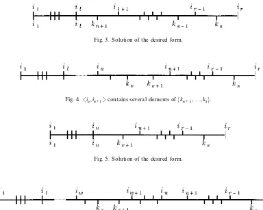
Fig. 3. Solution of the desired form.
Fig. 4. Si
u,iu`1Tcontains several elements ofMkn`1,2,ksN.
Fig. 5. Solution of the desired form.
Fig. 6. Siu,i
u`1Tdoes not contain any element ofMkn`1,2,ksN.
solution with more thanl!1 production periods.
Hence, DMk
duction periods for ELS(r) with at leastrelements.
Ifk
n`1toksare such that every setSil`t~1,il`tT
witht3M1,2,r!lNcontains exactly one of them,
then the just constructed optimal solution has the
desired properties (withm"l) (Fig. 3).
Otherwise, let u be the largest index in
Ml,2,r!1Nsuch thatSiu,iu`1Tdoes not contain
exactly one element ofMk
n`1,2,ksN. First, suppose
that Si
u,iu`1T contains several of these indices
and let k
v and kv`1 be the two largest of those
(Fig. 4).
Becausei
u is an optimal predecessor ofiu`1and
k
vis an optimal predecessor ofkv`1, it follows from
Lemma 1 thati
uis an optimal predecessor ofkv`1.
HenceMi
1,2,iuNXMkv`1,2,ksNis also an optimal
set of production periods. Moreover, this solution
has the form stated in the theorem (with m"u)
(Fig. 5).
Now, we are only left with the case thatSi
u,iu`1T
does not contain any element of Mk
n`1,2,ksN.
By deducing a contradiction, it will be shown that this case cannot occur. From the fact
that DMi
1,2,ilNXMkn`1,2,ksND*r we obtain
DMk
n`1,2,ksND*r!l. Therefore, there must be at
least one t3Ml,2,r!1NCMuN such that Sit,it`1T
contains several elements of Mk
n`1,2,ksN. From
the de"nition of uit follows that indices with this
property must be smaller than u. Let
w3Ml,2,u!1Nbe the largest index with the
prop-erty and letk
zandkz`1be the two largest indexed
elements inSi
w,iw`1T(Fig. 6).
It follows from the de"nition ofuandwthat for
allt3Mw#1,2,r!1Nthe setSit,it`1Tcontains at
most one element of Mk
Si
u,iu`1Tdoes not contain any element of the latter
set, it is now easy to show that
DMi
1,2,ilNXMkn`1,2,kzND
"DMi
1,2,ilNXMkn`1,2,ksND!DMkz`1,2,ksND
*r!(r!w!1)"w#1.
Furthermore, it follows from Lemma 1 that k
z
is an optimal predecessor of i
w`1. Hence,
not have an optimal solution with more than
wsetups forj
r. Hence, we have obtained a
contra-diction. This completes the proof. h
Theorem 1 is basically a characterization of how
the set of optimal production periods changes*or
to be more precise, may be assumed to change
*whenjbecomes equal toj@. Letrbe the smallest
index such thatj
r"j@, then there exists an optimal
solution with exactly q#1 setups of which the
production periods beforei
rare as described in the
theorem and the other production periods arei
r to
i
q. This characterization resembles a result given by
Murphy and Soyster [6], who consider the lot-sizing problem in which the setup and unit produc-tion costs are non-increasing over time, and the holding costs in each period are concave and non-decreasing functions of the inventory level at the end of that period. They show that when all setup
costs are decreasedproportionally(instead of by the
same amount), then the number of production
periods is non-decreasing and the kth production
period in the perturbed problem instance occurs
not later than the kth production period in the
original instance.
We now turn to the issue of determiningj@and
a corresponding optimal solution withq#1 setups
e$ciently. As noted before, we will determine the
values j
t, 2)t)q#1, in order of increasing
index. To explain our method we need some
addi-tional notation. For every pair of indices t
1 and
j"0 of the lot-sizing problem with planning
horizon consisting of the"rsti
r!1 periods
un-der the restriction that exactly one setup occurs
in Si
t,it`1] for all t3M1,2,r!2N, and j is the
only production period inSi
r~1,irT.
The reason why these values are introduced is the
following. Let r3M2,2,q#1N and suppose
jr(j
r~1. Consider a "xed j3Sir~1,irT and note
that the restriction in the de"nition ofG(j) makes
the corresponding optimal solution a candidate for the solution described in Theorem 1. Because this
solution has r setups, its value equals G(j)!rj
r
whenj"j
r. Clearly, the optimal solution of
The-orem 1 is the best one among all candidates, i.e., its value is min
Note that (3) holds under the assumption that
j
r(jr~1. Becausejr)jr~1, jr equals minMjr~1,
min
j|Wir~1,irXMG(j)N!F(ir!1)N, unless this value is
greater than K. In the latter case j
r is set equal
0,0. Note that the latter values are de"ned with
respect to the planning horizon with total demand
equal to d
1,ir~1~1. Therefore, the following
recur-sion holds:
The minimization in (4) determines an optimal
pre-decessor ofjin the restricted problem
correspond-ing to G(j). Because the last two terms do not
depend onh, we are mainly concerned with
calcu-lating the values min
h|Wir~2,ir~1+MG(h)#chdir~1,j~1N
for all j3Si
r~1,irT. To this end, we construct the
lower envelope of the lines with constant termG(h)
and slope c
h for h3Sir~2,ir~1]. For a "xed
j3Si
evaluating the lower envelope in coordinate
d
ir~1,j~1on the horizontal axis. Using similar
argu-ments as in Section 1, one can easily show that determining min
h|Wir~2,ir~1+MG(h)#chdir~1,j~1N in
this way for allj3Si
r~1,irTtakes a computational
e!ort that is bounded by a constant times the sum
of the cardinalities of the sets Si
r~2,ir~1] and
Si
r~1,irT. Subsequently, the valuesG(j) are easily
obtained for all j3Si
r~1,ir]. One can now
deter-minejrand proceed with the analogous calculation
ofG(k) for allk3Si
r,ir`1T. The complexity of this
algorithm to determinejq`1, and thus j@, is easily
seen to be O(¹). Note that a solution withq#1
setups that is optimal forj"j@can be constructed
in linear time if we have stored an optimal
prede-cessor ofjwhen calculatingG(j). To summarize, we
have the following result.
Theorem 2. It takes linear time to calculatej@(or to
xnd out that it does not exist)and to determine a solu-tion with exactly q#1 production periods that is optimal for thisvalue.
We have only looked at the parametric problem in which all setup costs are reduced when the para-meter increases. It is left to the reader to verify that similar results as presented in this section hold for the parametric problem in which all setup costs increase by the same amount when the parameter increases. Therefore, we state the following theorem without proof.
Theorem 3. Consider an economic lot-sizing problem without speculative motives that has an optimal solu-tion with q'1 production periods. Let jA be the smallest amount such that there exists an optimal solution with less thanqproduction periods when all setup costs are increased byjA. Thevalue ofjA and a corresponding optimal solution with exactlyq!1
setups can be determined in linear time.
4. Improved algorithms and theoretical results
In this section we show that the results obtained in Section 3 are not only interesting by themselves,
but that they also lead to improved algorithms for several problems which have been discussed before in the literature. Furthermore, we are able to gener-alize two known convexity results.
4.1. Computing stability regions
Richter [7,8] considers the economic lot-sizing
model with stationary cost coe$cients, i.e.,
f
i"f*0,hi"h*0 andpi"pfor alli3M1,2,¹N.
Without loss of generality, we may assume p"0
and therefore only the values offandhare relevant.
It is easily seen that not the absolute value of these
coe$cients, but rather their ratio determines the
optimal solution. Hence, the non-negative
quad-rant of the (f,h)-space can be partitioned into
con-vex cones, each of which corresponds to another
optimal solution. Moreover, there are at most¹of
these cones, each corresponding to another number
of setups in the optimal solution. For"xedf
0and
h
0and a given optimal solution Richter determines
the corresponding convex cone (`stability regiona)
using an algorithm that runs in at least O(¹2) time.
Van Hoesel and Wagelmans [9] point out that this time bound can actually be achieved. However, Theorems 2 and 3 imply an even stronger result. To
use those theorems we"x the unit holding cost to
h
0 and consider the two parametric problems that
result when j is subtracted from f
0, respectively,
added tof
0. Bothj@andjA, de"ned as before, can
be calculated in linear time. It is easily seen that the
given solution is optimal for all pairs (f,h) that
satisfy (f
0!j@)/h0)f/h)(f0#jA)/h0, and not
for any other pair. Hence, computing the stability region can be done in linear time, which is as fast as solving the problem.
We also note that if the setup cost is stationary, whereas the marginal production costs and holding costs are non-stationary, then the setup cost stabil-ity region (interval) can still be computed in linear time, provided that there are no speculative mo-tives. This constitutes a considerable improvement
over the O(¹3) algorithm of Chand and VoKroKs
[10], who only allow the holding costs to be
non-stationary. However, these authors also
4.2. Computing thevalue function and ezcient solutions
Zangwill [11] studies the implications of setup cost reduction in the economic lot-sizing model by performing a parametric analysis (see also [12,13]). His main motivation is to analyze the concepts of the Zero Inventory philosophy, which states that the inventory levels should be as small as possible and that this can be accomplished by reducing the setup costs. Zangwill shows that reducing all setup costs by the same amount may sometimes increase total holding costs. However, if the setup costs and
unit production costs are stationary (f
i"f and
p
i"pfor alli3M1,2,¹N), then setup cost reduction
leads to reduction of both the total holding costs and the number of periods with positive inventory.
Zangwill's results are partly based on the
analy-sis of thevalue function, i.e., the function that gives
the optimal value of the lot-sizing problem for
every j3[0,K]. It is easily seen that the value
function is piecewise linear, decreasing and
con-cave. Moreover, the function has at most¹linear
segments. To construct this function Zangwill
pro-poses an algorithm that runs in O(¹3). Instead of
this specialized algorithm one may use a well-known general method that is often attributed to Eisner and Severance [14]. This method constructs
the value function by solving at most 2¹#1
non-parametric lot-sizing problems. If the
Wag-ner}Whitin algorithm is used to solve the latter
problems again an O(¹3) time bound results.
How-ever, we may also use the linear time algorithm, because only lot-sizing problems without speculat-ive motspeculat-ives are considered. Hence, the value
func-tion can be constructed in O(¹2) time.
Theorem 2 implies yet another approach to con-struct the value function. We may apply the pro-cedure given in Section 2 repeatedly. Starting with
an optimal solution forj0,0, we"rst"ndj@, the
largest value of j for which the given solution is
optimal. At the same time we"nd a solution that is
optimal forj@and that has one setup less than the
original optimal solution. We now proceed by
letting j@play the role of j0. Clearly, we will"nd
the complete value function after at most ¹!1
applications of our procedure. Hence, this
ap-proach also takes O(¹2) time, and from a
complex-ity point of view it does not perform better than the
Eisner}Severance method. However, in the
follow-ing application this approach is particularly useful. Richter [15] analyzes the stationary cost model with respect to the criteria total costs and total
inventory. The goal is to"nd allezcient solutions,
i.e., all solutions for which there does not exist another solution that is better on one criterion and not worse on the other. Assume that the there exists an optimal solution (w.r.t. total costs) that has
q(¹production periods. One can show that the
total inventory is non-increasing in the number of setups; for instance, this follows from the result by Zangwill [11] mentioned earlier and also from
Theorem 4 in the next subsection. Hence, to"nd all
e$cient solutions it su$ces to determine for all
k3Mq,2,¹Nthe optimal value of the problem in
which the number of setups is restricted to be
exactlyk. The latter can be done by calculating the
value function of the parametric problem in the
way indicated above (where K equals the setup
cost). This approach has a lower running time than the one used by Richter, which is based on the
Wagner}Whitin algorithm and runs in O(¹3) time
or worse (no complexity analysis is given). We
should also mention that the Eisner}Severance
method can not be used, because it does not
neces-sarily determine optimal solutions for all
k3Mq,2,¹N. In particular the latter may happen if
for somek3Mq,2,¹Nthe corresponding solution
is only optimal for one value ofj3[0,K].
4.3. A convexity result
Consider a lot-sizing problem without speculat-ive motspeculat-ives and suppose that there exists an
opti-mal solution with q'1 setups. For k3M1,2,¹N
we let TC(k) denote the optimal value of the
prob-lem in which the number of setups is restricted to be
exactlyk.
Theorem 4. The function TC is non-increasing on
M1,2,qN and non-decreasing on Mq#1,2,¹N. Furthermore, TCis convex onM1,2,¹N.
Proof. We will provide the proof only for the range
M1,2,qN. A similar proof holds for the other range
Consider the parametric problem in which the
setup cost in periodiis equal tof
i#K!j, where
j3[0,K] and K"c
1d1T. Hence, for j"K there
exists an optimal solution with q setups and for
j"0 it is optimal to produce only in period 1. It
follows that there exist values 0"j0)j1)2)jq
"K such that for every k3M1,2,qN there are
k setups in an optimal solution if and only
if j3[jk~1,jk]. The value of an optimal solution
with k setups is equal to TC(k)#kK!kj. For
j"jk, 1)k(q, optimal solutions with k and
k#1 setups exist. Therefore,
TC(k)#kK!kjk"TC(k#1)#(k#1)K
!(k#1)jk
or equivalently
TC(k)!TC(k#1)"K!jk. (5)
Because the right-hand side of this equality is non-negative, it follows that TC is non-increasing on
M1,2,qN. Clearly, for 1(k(qit also holds that
TC(k!1)!TC(k)"K!jk~1.
Combining this with (5) andjk~1)jk, we obtain
TC(k)!TC(k!1))TC(k#1)!TC(k)
and this means that TC is convex onM1,2,qN. h
Remark. Note that the problem reformulation that we have carried out (eliminating the holding costs
and replacing p
i byci) does not a!ect this result,
because it has caused the value of all feasible solu-tions to change by the same amount. For
conveni-ence, we assume that TC(k) equals the solution
value w.r.t. the original objective function.
An obvious application of Theorem 4 concerns the problem in which the number of setups is
restricted to be at mostn. The theorem states that if
the unrestricted problem has an optimal solution
withq'nproduction periods, then there exists an
optimal solution of the restricted problem with
exactly n setups and it follows from the proof of
Theorem 4 that this solution can be determined in
O(n¹) time.
Theorem 4 generalizes a result by Tunc7el and
Jackson [16], who use a completely di!erent
ap-proach to show this result for the special case in
whichp
i"pfor alli3M1,2,¹N. It also generalizes
a result by Chand and Sethi [17], who also consider the special case of stationary marginal
production costs. They de"ne HC(k) to be the
minimum holding cost if the number of setups is
restricted tok3M1,2,¹Nand show that this
func-tion is non-increasing and convex. To see that this
is a special case of Theorem 4, it su$ces to assume
f
i"pi"0 for alli3M1,2,¹Nand to note that in
that case q"¹ and TC(k)"HC(k) for all
k3M1,2,¹N.
5. Concluding remarks
By carrying out a parametric analysis of the setup costs in the economic lot-sizing problem, we have obtained new results about the structure of optimal solution for given number of setups, we have been able to design fast algorithms for several related problems and we have obtained additional theoretical results which may be useful. Our analy-sis and the algorithms which we have proposed
di!er signi"cantly from existing approaches. We
think that the characterization given in Theorem 1 and the algorithm it suggests are particularly interesting. An interesting topic for future research is the question whether similar results hold if we allow backlogging.
Acknowledgements
Part of this research was carried out while the second author was visiting the Operations Re-search Center at the Massachusetts Institute of
Technology with"nancial support of the
Nether-lands Organization for Scienti"c Research (NWO).
He would like to thank the students, sta! and
faculty a$liated with the ORC for their kind
hospitality.
References
[2] A. Federgruen, M. Tzur, A simple forward algorithm to solve general dynamic lot sizing models withnperiods in O(nlogn) or O(n) time, Management Science 37 (1991) 909}925.
[3] A. Wagelmans, S. Van Hoesel, A. Kolen, Economic lot-sizing: An O(nlogn) algorithm that runs in linear time in the Wagner}Whitin case, Operations Research 40 (1992) S145}S156.
[4] S. Van Hoesel, A. Wagelmans, B. Moerman, Using geo-metric techniques to improve dynamic programming algo-rithms for the economic lot-sizing problem and extensions, European Journal of Operational Research 75 (1994) 312}331.
[5] H.M. Wagner, T.M. Whitin, Dynamic version of the eco-nomic lot size model, Management Science 5 (1958) 89}96. [6] F.H. Murphy, A.L. Soyster, Sensitivity analysis of the costs in the dynamic lot size model, AIIE Transactions 11 (1979) 245}249.
[7] K. Richter, Stability of the constant cost dynamic lot size model, European Journal of Operational Research 31 (1987) 61}65.
[8] K. Richter, Sequential stability of the constant cost dynamic lot size model, International Journal of Produc-tion Economics 34 (1994) 359}363.
[9] S. Van Hoesel, A. Wagelmans, A Note on&&Stability of the Constant Cost Dynamic Lot Size Modelaby K. Richter,
European Journal of Operational Research 55 (1991) 112}114.
[10] S. Chand, J. VoKroKs, Setup cost stability region for the dynamic lot sizing problem with backlogging, European Journal of Operational Research 58 (1992) 68}77. [11] W.I. Zangwill, From EOQ towards ZI, Management
Science 33 (1987) 1209}1223.
[12] W.I. Zangwill, Set up cost reduction in series facility pro-duction, Working paper, Graduate School of Business, University of Chicago, Chicago, IL, 1985.
[13] W.I. Zangwill, Eliminating inventory in a series facility production system, Management Science 33 (1987) 1150}1164.
[14] M.J. Eisner, D.G. Severance, Mathematical techniques for e$cient record segmentation in large shared databases, Journal of the Association for Computing Machinery 23 (1976) 619}635.
[15] K. Richter, The two-criterial dynamic lot size problem, System Analysis, Modelling, Simulation 1 (1986) 99}105.
[16] L. Tunc7el, P.L. Jackson, On the convexity of a function related to the Wagner}Whitin model, Operations Research Letters 11 (1992) 255}259.