SPATIAL DIFFERENTIATION OF SOCIOECONOMIC AND
INFRASTRUCTURE DEVELOPMENT IN RURAL’S MOUNTAIN AREA
A Spatial Approach for Rural Development Planning
Iwan Rudiarto1)andWiwandari Handayani2)
1)
Department of Urban & Regional Planning, Diponegoro University, Indonesia [email protected] / [email protected]
2)
Department of Urban & Regional Planning, Diponegoro University, Indonesia [email protected]
ABSTRACT
Spatial differentiation of available resources and socioeconomic conditions of rural populations has been contributing to farming system variety which directly affect to the farming families. Farming families are distributed in different locations along the gradual line of rural mountain areas; therefore, their characteristics are also different. These characteristics can be described within spatial methodologies by linking all the related data and information into spatial aspects. It would be a great challenge to describe more informative economic conditions as research in linking spatial setting on economic situation of the farmers is often disregarded in social sciences. Methodological problems in regional assessment of mountain farming system sustainability arise due to representative household surveys, which are bound to a certain scale in which they serve as models for a case. In a micro level survey, conditions of farm families are evaluated in detail only in limited number of surveyed households or villages and valid only for certain cases. But in a broader context, regionalization has become necessary to cover all related issues and problems for the whole study area. Therefore, this paper is purposed to overcome these issues through a spatial gradient analysis concept by looking at from two perspectives, i.e. socioeconomic conditions and road infrastructure development by conducting research in Dieng Plateau, Central Java. The result shows that socioeconomic conditions and road infrastructure development are differed one another following the concept and hence, further decision on development planning can be purposed.
Keywords: Socioeconomic, Road infrastructure, Mountain area, Dieng plateau
A.
INTRODUCTION
resources that may exist in their location. Families located at higher altitudinal levels generally coped with relative inclined areas and distance to economic centre. In this area, resources are somehow limited where physical conditions become the major constraint to be dealt with. In the middle area, the conditions are quite similar to the higher area but the constraints are normally found less than higher area. In some cases, issues and problems related to the agricultural activities appear at the same level as initiated in high and low level areas. At the same time, the lower area is able to provide more possibilities in terms of access and resources due to its location. Farm families living in this area will have more benefits in better agricultural systems as well as in associated matters. Resource availability and utilization have been contributing in shaping different gradations of socioeconomic development that is managed in different directions according to the spatial differentiation.
Since farming families are distributed in different locations along the gradual line of mountain areas, their characteristics are also different. These characteristics can be described within spatial methodologies by linking all the related data and information into spatial aspects. It would be a great challenge to describe more informative economic conditions as research in linking spatial setting on economic situation of the farmers is often disregarded in social sciences. Methodological problems in regional assessment of mountain farming system sustainability arise due to representative household surveys, which are bound to a certain scale in which they serve as models for a case (Lentes, 2003). In a micro level survey, conditions of farm families are evaluated in detail only in limited number of surveyed households or villages and valid only for certain cases. But in a broader context, regionalization has become necessary to cover all related issues and problems for the whole study area. To cover these matters, regional coverage can be applied to the sampling data following the concept of spatial gradient analysis. According to Doppler (2006), gradient analysis are those parameters in the space in the region which are reflections of the economic, social, administrative, political, cultural, and environmental conditions of the families and societies in the region. By following this concept, regionalization of sampling data is possible although spatial spread and sample size collected from the micro survey level does not meet the numbers for a regional level analysis. Therefore, this paper is purposed to describe socioeconomic conditions and road infrastructure development in mountain area by taking the case from Dieng Plateau, one of famous upland agriculture area in Central Java.
B.
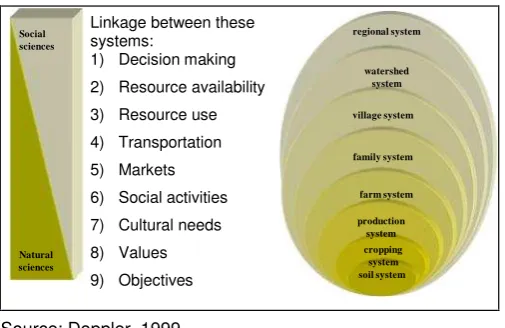
VERTICAL AND HIERARCHICAL CONCEPT IN FARMING SYSTEMS
hierarchy (Doppler, 1999). It means that two possibilities of widening scale in spatial analysis are exist, information can be collected either directly on the level of the hierarchy that is of interest of one step lower that the level of interest (K. C., 2005). Considering the provided collection data is a representative, therefore, it is possible to scaling these data up to the next level of the hierarchy. In this context, the collection of farm household data in selected study area has been possible to transfer the results from the family level into the population level and generate information for the specified study area.
soil system
Figure 1. The vertical linkages and hierarchy system in farming systems
In the mountain areas, land availability and farm size are quite complex in term of their interactions and site conditions. Specific forms and zones of land use and farm types are found according to their spatial location. These specific shapes of land use imply the seeking of spatial relationship dimensions in a family and society, which can be spatially described through spatial modeling. Relationship dimensions in this context could be in vertical or horizontal measurements. Interfacing of horizontal and vertical relationships into spatial distribution measurements is particularly relevant with regard to vertical linkages to facilitate the discouragement of spatial equity by placing the focus on the living standard of individual families. Due to different spatial locations of farm families within the society, the requirement of spatial methodology is necessary to bridge linkages and interrelationships within the overshadowed system.
C.
METHOD AND ANALYSIS
As this paper is intended to produce spatial description on socioeconomic and infrastructure development in Mountain area, spatial calculations were carried out. In socioeconomic analysis, an interpolation technique was applied to generate data for the whole study area while infrastructure development was assessed through a cost distance model.
estimating the value of a field variable at un-sampled sites within the area covered by sample locations or in simple words, given a number of whose locations and values are known (Zhang and Goodchild, 2002). It can be used to create a grid simply by estimating values at the centers of each grid cell. The understanding on how interpolated grid is created depends on the understanding how interpolation is performed at a single point. Data collection from every location in a study area to determine the height, magnitude or concentration of a physical property may not generally be practically feasible and economically viable. Therefore, interpolation is used to create a continuous surface, by acquiring new values of parameters at points that have not been directly sampled.
In order to generate values at the un-sampled sites, there are four interpolation techniques that can be applied, i.e.: Inverse Distance Weighted (IDW), Spline, Kriging, and Trend (Naoum and Tsanis, 2004). IDW interpolator assumes that each point has a local influence which is inversely proportional to a selected power of the distance. Spline is an interpolation method that estimates values using a mathematical function that minimizes overall surface-curvature and produce a smooth surface that passes through the input points. Kriging interpolator calculates the distance or direction between sample points to show spatial correlation that can help to describe the location. Trend interpolator fits mathematical function, a polynomial of specified order, to all input points. Figure 2 shows the different results of interpolation technique.
Figure 2. Interpolation techniques, a) IDW, b) Spline, c) Trend, and d) Krigging
Spatial interpolation technique has been applied to derive spatial information from tabular socio economic data into spatial data by linking the data to each corresponded family as explained before. Due to the function and the suitability of each interpolation method, Inverse Distance Weight (IDW) was selected to generate grid data in the un-sampled area. IDW method assumes that the variable being mapped decreases in influence with distance from its sampled location while spline method is best for gently varying surfaces such as elevation, water table heights, or pollution concentration (ESRI, 1996). Krigging method
a) b)
involves several steps in its process and more appropriate used if the user has already known the spatially correlated distance or directional bias in the data. Trend interpolator as explained above only fits into the mathematical function and stressing the regression model.
IDW method determines the output values for each location from all points within a specified radius. This technique creates weights according to the distances between the interpolated location (x,y) and each neighbors. The calculation of using this method is derived from the weighting mathematical function which can be described as (Shekhar and Xiong, 2008):
Where, w(x,y) is the predicted value at the location (x,y),n is the number of nearest known points surrounding (x,y),λiare the weights assigned to each known point valuewiat location (xi, yi),diare
the 2D Euclidean distances between each (xi,yi) and (x,y), andp is the exponent, which influences
the weightingwionw.
Cost Distance Analysis
Basically, the application of cost distance modeling is assembled from ESRI (1996) which was introduced to calculate weighted distance mapping for the least costly road through specific landscape. Cost distance model applies distance as a unit cost not in geographic units. Cost units in cost distance model can be interpreted as monetary units as well as time units. A cost grid assigns an impedance factor in some uniform measurement system to depict the cost of moving through an individual cell (ESRI, 1996). Each cell has its own cost value and assumed to represent the cost per unit distance of passing trough the cell in the area where each unit distance corresponds to the cell width.
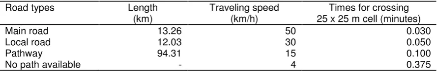
Table 1. Available road infrastructure in study area
time required to pass each road. The traveling time was estimated from the transportation standard of speed for different road classification in Indonesia for hilly area as well as from the field measurement and own experience.
Each type of road was weighted according to its capability speed to be traveled as shown in Table 1. Different weighted values were given for each 25 x 25 m cell which means for instance; on the main road the weighted value is 0.030 minutes because it will take 1.8 seconds to cross one cell with 50 km/h of traveling speed. This calculation is also applied for other types of road and particularly for the areas where no road available, the traveling speed was set up to 4 km/h based on walking speed assumption. With all weighted values then the road map was converted into the grid form where the analysis of cost distance will be performed. Since study area is a mountainous area, inclination also influences the traveling speed from one area to another. Therefore, inclination is needed to be considered as the influencing factor in determining the traveling speed. Weighted grid map was created through the slope map which is generated from Digital Elevation Model. Slope map is grouped into five classifications adopted from Departemen Kehutanan (1998) and each group was weighted according to this class. The given weight values in this map are laid between 1 for the flat areas and 2 for the very steep slopes above 40%, the less the slope and the less weighted value will be given.
Source: Author based on ESRI, 1992
Figure 3. Accumulative cost calculation, a) horizontal and vertical, and b) diagonal
To produce the cost grid map, the weighted road and slope map were multiplied through the map calculation. As the result, the cost grid map represents the time needed for crossing the cell and indicated as the z value for each cell distributed in the whole study area. Afterwards, this cost grid map is assessed through the cost distance option by considering the specific location as the source map, in this study district centre and the multiplied cost grid map. In cost distance, the shortest route between two points may not be the straight line and even if it is straight, its geographical length may not always reflect a meaningful measure of distance. To a certain extent, distance in this application is best defined in terms of movement expressed as travel time, cost, or energy that may be consumed at rates that vary over time and space (Berry, 1997).
D.
RESULTS AND DISCUSSION
Socioeconomic Characteristics
By using IDW method in interpolating socioeconomic data from sampled points, all the unknown value of un-sampled area within the study area are able to be identified. The interpolation has been done through nearest neighbors with 12 sample points option and power functions of 2. However, the interpolation results may over or underestimate the conditions at the edge of surface. The interpolation, particularly at the border of study area and at the less sample point area, is often continued with unrealistic values. Once the last sampling point is passed, the derived trend continues with the same gradient as before the sampling point and makes the values rise or decline inappropriately in some cases. To avoid these possible errors, the interpolated grid layers were classified, thus only the class bandwidth is readable from the maps (Lentes, 2003).
Figure 4. Interpolation results of selected socioeconomic variables a) farm income, b) weighted education index, c) family income, d) potato yield, Dieng Plateau, 2006
As for example of interpolation results from the total of 75 interviewed families, Figure 4a, 4b, 4c, and 4d show the spatial distribution of farm income, weighted education index,
a) b)
family income, and potato yield in study area. Farm income level is quite high in high altitude area compared to those surveyed family in middle and lower area. But for some extends, farm income level in low area is higher than middle area due to the high level production of potato and vegetables and the size of farmland which is bigger than middle area. On the other hand, the interpolation of weighted education index in study area shows more educated people in lower area compared to those in higher area. Spatial distribution of educated people clearly shows that higher level of education attainment lied along and around the most accessible part which is indicated by the road. Family income is higher in high altitude area and some part of middle altitude area. At the same time, low level of family income is to be more found in low altitude area as well as some part of middle altitude area. The spatial distribution of potato yield clearly shows that high area has more yields on potato per hectare than other areas. The distribution also describes that the tendency of potato yield decreases to the lower area. It might be happened due to the production potential of available land resources where high land has more potency to grow potato. However, high level of the yield does not only depend on the available land resources but also other related factors such as production inputs and the ability of farmers in maintaining their farmland from external disturbance such as plant disease and soil loss.
Road Network Analysis
Cost distance estimations support the best possibilities to provide more detailed and more consistent information in term of distance calculations. Cost distance modified the distance concept by applying flexible weights and used reasonable cost raster dataset by adding weight into the distance between different points. Cost can be adjusted into different units whether it is time unit or monetary unit and calculated as the result of accumulative cost function as shown in Figure 5.
Figure 5. Cost distance to the district centre, Dieng plateau 2006
distance. Since the cost grid surface refers to the specific location, i.e.: district centre, the area near by that location will consequently have the less cost distance unit. Cost distance appears differently when altitude level is being concerned and gives varieties on the accessing time from household samples to the district centre. The comparison between higher and lower altitude areas will consequently perform different capability and ability of the surveyed family in term of accessing all the public services provided in district centre as well as in reaching important parts of available inputs for farming activities and off farm sector.
Table 2. Average access time from household samples to district centre (in minutes) Dieng plateau, 2006
Cost distance statistics Low area Middle area High area
Average 24.30
(±10.88)
22.38 (±4.73)
48.26 (±6.50)
Highest cost distance value 106.4 41.80 79.40
Lowest cost distance value 0.80 0.50 30.30
Differences between (1) and others - ** **
Differences between (2) and others - -
-Figures in Parentheses are mean values at 95% confidence of interval. Probability that the hypothesis of non significant differences among the groups can be rejected according to the Mann-Whitney test: ** ≤ 99%
As described in Table 2, the cost distances are differed significantly from three different group areas, i.e.: low area, middle area, and high area. In low area the average time to reach the district centre is 24.30 minutes while middle area 22.38 minutes and high area 48.26 minutes. Due to the location of district centre in middle area, cost distances for higher and lower area are greater than those closer to the centre. High area is more than double in minutes to reach the centre compared to the low and middle area. Concerning the highest cost distance values, low area is found to have the highest value followed by high and middle area. On the other hand, middle area is indicated as the lowest time in cost distance followed by low and high area. According to the significant test, middle area and high area have significant different in term of the average values. These differences might occur due to the infrastructure and distances related constraints in mountainous areas.
Road Networks Improvement and Development
condition and hence improvement at the time being is considered unnecessary. Besides, the responsibility to maintain this road is under regional authority, i.e. province and national level. Therefore, all issues concerning road improvement and development should fulfill certain conditions which need more time to decide.
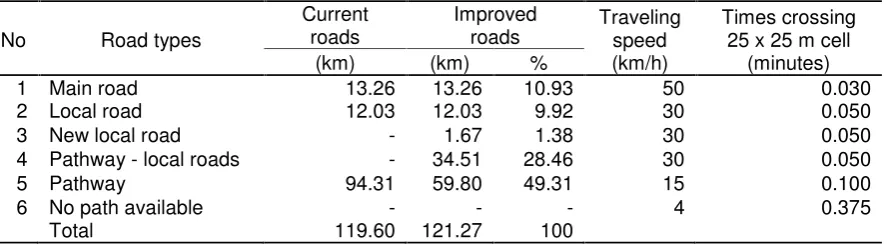
Table 3. Current and improved road networks in study area
No Road types
1 Main road 13.26 13.26 10.93 50 0.030
2 Local road 12.03 12.03 9.92 30 0.050
3 New local road - 1.67 1.38 30 0.050
4 Pathway - local roads - 34.51 28.46 30 0.050
5 Pathway 94.31 59.80 49.31 15 0.100
6 No path available - - - 4 0.375
Total 119.60 121.27 100
As shown in Table 3, improved road was proposed for about 34.51 km by enhancing the function of pathway into local road which automatically improve the road class. This road improvement was located in ten villages and mostly distributed in middle and high area, e. g.; Buntu, Sigedang, Igirmranak, Surengede, Jojogan, Patakbanteng, Sembungan, Sikunang, Campursari, and Serang. Meanwhile, new local road was developed for about 1.67 km that connected higher area and middle area. With this improvement, therefore, local road in study area was extended for about 36.81 km from current road and pathway has been reduced for 34.51 km or 28.46% from total road length. Higher road class, main and local road, dominated for about 50.69% which indicates the level of better accessibility provided in study area. Moreover, new and improved roads were mainly proposed in vital areas where farmers would have more access to certain areas, particularly farm field. At the end, road improvement and development is able to enhance traveling speed from one to another area and therefore increasing the productivity and activity movement.
Cost distance with road improvement and development
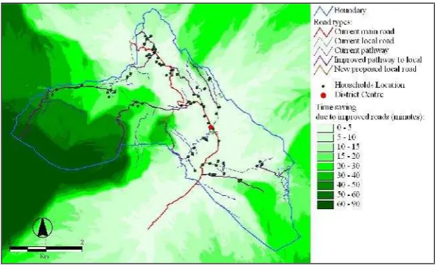
To portray benefit of road improvement and development in study area, a cost distance measurement was employed. This measurement is able to show the enhancement of accessibility upon the proposed road network scenario. As the result, different cost units in minutes from district centre to each grid cells unit covering study area are described as shown in Figure 6.
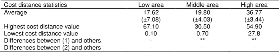
traveling time can be saved more than 20 minutes, precisely up to 90 minutes. This is due to the enhancing road class in those areas that significantly decreasing traveling time.
Figure 6. Cost distance with road improvement and development
Figure 7. Time saving under road improvement and development compared to the current cost distance
Table 4. Average access time from household samples to the district centre
Cost distance statistics Low area Middle area High area
Average 17.62
(±7.08)
19.80 (±4.03)
36.77 (±3.44)
Highest cost distance value 67.10 30.50 54.90
Lowest cost distance value 0.10 0.70 27.8
Differences between (1) and others - ** **
Differences between (2) and others - -
-Figures in Parentheses are mean values at 95% confidence of interval. Probability that the hypothesis of non significant differences among the groups can be rejected according to the Mann-Whitney test: ** ≤ 99%
E.
CONCLUSIONS
The identification of socioeconomic condition is more clearly distinguished between one region and another by applying spatially description analysis where data are not only described into tabular form but also into spatial context. In general, it can be concluded that spatial description from the interpolated map shows the relation of socioeconomic development among the region in study area and can be distinguished explicitly based on the altitudinal level of household samples such as high, middle, and low area as study area located on a mountainous region. The interpolated maps and autocorrelation results, obviously can help the understanding of related policy makers/stakeholders on how the socio economic distributed in spatial level. Therefore, the descriptions of problems, potentials, and advantages of study area can be clearly identified, and then the decisions on further rural development policies can be proposed with respect to the results.
In relation to road infrastructure development, cost distance analysis showed some differences in term of possible source between areas in farm and off-farm incomes. The availability of off farm employment and possibilities of buying inputs and products as well as to sell the products in district centre are some of the examples related to the gradients associated with cost distances. Regarding this fact, therefore, accessibility has become further interest to be prioritized as constrains and potentials for rural development in study area closely related to the infrastructure issue. In a simple term, the easiness in accessing all destinations in one region is very much depend on the availability of the infrastructure, quantitatively as well as the quality. Through different improvements of road networks then several impacts to socioeconomic development can be envisaged. These improvements may consider different scales whether local or regional scale. At the local level, road improvement is tend to open access in specific areas and creates the easiness of movement from farm filed to the local centre. On the other hand, regional improvement and development of road networks are able to create mobility among people and activities centre, particularly related to economic movement of goods and services. By considering different scales, a better condition of rural development would be achieved.
F.
REFERENCES
Departemen Kehutanan. 1998. Pedoman Penyusunan Rencana Teknik Rehabilitasi, Teknik Lapangan dan Konservasi Tanah Daerah Aliran Sungai. Departemen Kehutanan. Jakarta. [Ref type: Regulation]
Doppler, W. 1999. Setting the Frame: The Environmental Perspectives in Rural and Farming System Analyses, In Doppler, W., and Koutsouris, A. eds. Rural and Farming System Analyses: Environmental Perspective. Margraf Verlag. Wekersheim. [Ref type: Book]
Doppler, W. 2006. Resources and Livelihood in Mountain Areas of South East Asia: Farming and Rural Systems in a Changing Environment. Margraf Verlag. Wekersheim. [Ref type: Book]
Direktorat Jenderal Bina Marga/DJBM. 1997. Tata Cara Perencanaan Geometrik Jalan Antar Kota. DJBM. Jakarta. [Ref type: Regulation]
Direktorat Jenderal Bina Marga/DJBM. 1997. Manual Kapasitas Jalan Indonesia (MKJI). DJBM. Jakarta. [Ref type: Regulation]
ESRI. 1996. ArcView Spatial Analyst: Advanced Spatial Analysis Using Raster and Vector Data. Environmental System Research Institute. Redlands. California. [Ref type: Book]
ESRI. 1996. ArcView GIS: The Geographic Information System for Everyone.
Environmental System Research Institute. Redlands. California. [Ref type: Book]
K. C. Khrisna, Bahadur. 2005. Combining Socio-Economic and Spatial Methodologies in Rural Resources and Livelihood Development: A Case From Mountains of Nepal. In: Doppler, W., and Bauer, S., (Eds.) Farming and Rural System Economics Vol. 69. Universität Hohenheim, Dissertation. Margraf Verlag. Wekersheim. [Ref type: Book]
Lentes, P. 2003. The Contribution of GIS and Remote Sensing to Farming System Research on Micro- and Regional Scale in North West Vietnam, In: Doppler, W., and Bauer, S., (Eds.) Farming and Rural System Economics Vol. 52. Universität Hohenheim, Dissertation. Margraf Verlag. Wekersheim. [Ref type: Book]
Naoum, S. and I. K. Tsanis. 2004. Ranking Spatial Interpolation Techniques Using a GIS-Based DSS. In: Global Nest. Vol. 6. No. 1. pp. 1-20. Greece. [Ref type: Journal]
Rudiarto, I. and Doppler, W. 2009. Integrating Socioeconomic Development into Spatial Modeling in Indonesian Upland Agriculture: A case of Dieng plateau, Central Java – Indonesia. Paper Presented at: European Agricultural Economist Association (EAAE) PhD Workshop. September 10th– 11th, 2009. Gießen. Germany. [Ref type: Paper]
Shekhar, S. and Xiong H. 2008. Encyclopedia of GIS. Springer Verlag. Berlin. [Ref type: Book]