Government Spending on Infrastructure in
an Endogenous Growth Model with Finite
Horizons
Iannis A. Mourmouras and Jong Eun Lee
This paper examines the effects of government spending on infrastructure within an endogenous growth model populated by consumers with finite horizons. It highlights the role of finite horizons in such a framework, and also compares and contrasts the effects of government spending on macroeconomic performance and individual utility with those obtained in the infinite horizon representative model. © 1999 Elsevier Science Inc.
Keywords: Uncertain lifetimes; Public investment; Barro curve JEL classification: H54, O41
I. Introduction
Following the influential work of Barro (1990), a rapidly growing literature has sprung up in macroeconomics investigating the long-run effects of public investment on macroeco-nomic performance. A number of researchers [for instance, Barro and Sala-i-Martin (1992); Baxter and King (1993); Futagami et al. (1993); Turnovsky and Fisher (1995)] have recently developed models in which governmental activities, in the form of provision of infrastructural services, affect the long-run growth rate of the economy through the production function, as a factor along with private capital. The general idea behind having productive government services as an input to private production is that private inputs are not a close substitute for public inputs. The main theoretical prediction of this literature is that increases in government spending on infrastructure are associated with higher long-run growth rates; however, this rise in the growth rate is reversed after a point (the hump-shaped Barro curve), showing that there is an optimum value for public investment.
Department of Economics, School of Management, Heriot-Watt University, Edinburgh, United Kingdom; Department of Economics, Seoul National University, Seoul, Korea.
Address correspondence to: Dr. I. A. Mourmouras, Department of Economics, School of Management, Heriot-Watt University, Edinburgh, EH14 4AS, UK.
Moreover, a number of recent quantitative studies have attempted to measure the effect of public infrastructure on output growth. For instance, Aschauer (1989), in his study for the United States (1949 –1985), found that government spending on infrastructure, among other forms of investment, has maximum explanatory power on the productivity of private capital. Baxter and King (1993) calibrated a model economy for the United States, and they also found that publicly-provided capital has substantial effects on output and private investment. Easterley and Rebelo (1993), too, found that the share of public spending in transport and communications had a robust correlation with growth in their cross-section data set of about 100 countries for the period 1970 –1988. In brief, empirical evidence also suggests that services from government infrastructure are quite important for output growth.
Most of the recent theoretical work on the role of public investment has been done within an endogenous growth1framework, as the emphasis is on long-run effects. As is well known, in the old growth theory, growth at the steady state is determined entirely by technology [Solow (1956)], and the real interest rate depends only on preferences, i.e., the modified golden rule [Cass (1965)]. In contrast, in the endogenous growth theory [Romer (1986); Rebelo (1991)], the growth rate is always a function of preferences and technol-ogy, and the real interest rate in addition to preferences may also depend on technology. Kocherlakota and Yi (1996, 1997), among others, have recently made a genuine attempt to empirically distinguish between endogenous and exogenous growth models by using their differing implications for the long-run effects of government policy changes on growth rates. Their results lend support to endogenous growth models, especially those which include productive non-military structural capital. In this paper, we examine the effects of government spending on infrastructure within an endogenous growth model populated by consumers with uncertain lifetimes. Our framework combines the Blanchard (1985) overlapping generations (OLGs) model with the endogenous growth model devel-oped by Barro (1990). Thus, like Barro, within the broad concept of capital, we consider tax-financed government services that affect production. Our main objective is to high-light the role of finite lives within the above framework and, as Barro’s infinite horizon framework can be obtained within our model as a limiting case, to contrast and compare the results of the finite lives model with those obtained in the infinite horizon represen-tative model of endogenous growth. This is a non-trivial task because, with finite horizons, the effects of public investment are bound to be quite different due to the different wealth effects on consumers.
The structure of the paper is as follows: In Section II, we present a simple model of optimal savings and endogenous growth. Section III derives and characterizes the steady state, and also discusses the implications of finite horizons. Section IV investigates the macroeconomic effects of a balanced budget rise in government spending on infrastruc-ture with finite and infinite horizons. Section V offers some concluding remarks.
II. The Model
In this section, we present a model which combines the overlapping generations model of Blanchard (1985) with the endogenous growth model of productive government services
developed by Barro (1990). The Blanchard (1985) framework is an exogenous-growth model, while Barro (1990) assumes a representative infinitely-lived household. The novel element in our model is to combine2 the Blanchard type of consumers with uncertain lifetimes with the Barro type of producers who benefit from government spending on infrastructure. Time is assumed to be continuous.
The Individual Consumer and Aggregation
The consumption side of the model is a version of the perpetual-youth overlapping-generations framework proposed by Blanchard (1985). The economy consists of a large number of identical households, born at different instances in the past and facing a constant probability of death,l(0#l). At any point in time, a large generation is born, the size of which is normalized tol.lis also the rate at which the generation decreases. Thus, a generation born at time zero has a size, as of time t, ofle2lt. Aggregation over generations then implies that the size of population at any point in time is equal to 1. A household born at time zero is alive at time t, with probability e2lt, which implies that its expected lifetime is just 1/l. As l goes to zero, 1/l goes to infinity: we then say that households have infinite horizons.
Following Blanchard (1985), we also assume that there is no intergenerational bequest motive. Because of the probability of death and the absence of any bequest motive, there is a role for a market for insurance in this framework in order to account for those who die in debt or those who die with positive assets.3 The two assumptions of a constant probability of death and the existence of life-insurance companies which provide insur-ance in the form of annuities to agents contingent on their death, taken together, tackle the problem of aggregation.4
Thus, individual i, born at time s, chooses a consumption plan to maximize her expected lifetime utility:
where cidenotes consumption of household i, andr is the rate of time preference. Cass
and Yaari (1967) have shown formally that the effect of the probability of death is to increase the individual’s rate of time preference (intuitively, the higher the probability of death, the more heavily one discounts the future).
The household’s dynamic budget constraint is given by:
dai~s,t!
dt 5@r~t!1l#a
i~s,t!1v~t!2ci~s,t!, (2)
2Thus, our framework is close to that developed by Saint-Paul (1992), who also combined Blanchard-type consumers with an endogenous growth model (in his case, it was the AK model, and he did not consider productive government services).
where ai denotes asset wealth; v(t) is the (net) instantaneous non-asset income of the household, and r(t) is the real interest rate. We assume that the representative household supplies labor inelastically (e.g., say, one unit of labor), for which she receives a payment
v(t). Note that, following Blanchard (1985) we assume that newly-born individuals do not inherit any asset wealth and that labor income, v, is independent of the age of the household. It is also assumed that the transversality condition which prevents consumers from going infinitely into debt is satisfied. The optimization for the individual consumer then yields:
dci~v!
dv 5@r~v!2r#c
i~v!. (3)
Integrating both equations (2) and (3), and combining them yields:
ci~t!5~r 1 l!@ai~t!1hi~t!#, (4)
where hi(t) denotes individual human wealth, interpreted as the present discounted value of labor income.5 The above equation simply states that individual consumption is proportional to human and non-human wealth, with propensity to consume (r1l), which is independent of age. Aggregation over generations can then be done in the following manner:
where X(t) represents an aggregate variable, and x(s,t) denotes its individual counterpart for an agent born in s, as of time t. Using the above procedure, one can obtain aggregate consumption (after eliminating human wealth):
dC~t!
dt 5@r~t!2r#C~t!2l~r 1 l!A~t!, (6) where capital letters denote economy-wide aggregates. Note that with the assumption of finite lives (i.e.,l . 0), the rate of change of aggregate consumption depends on asset wealth. This is not the case for the infinite horizon case (i.e., whenl 50).
Producers
The production side of the model follows closely the Barro (1990) framework of productive government services. The government purchases a portion of the private output produced in the economy, and then uses these purchases to provide free public services to a single representative firm which stands in for a competitive industry. In other words, such productive services are complementary to private capital, something which raises the long-run growth rate of the economy. Let G be the quantity of productive government
services measured in terms of the (single) good produced in the economy. We assume that these services are nonrival for the users (and, hence, the model abstracts from the Barro and Sala-Martin (1992) congestion type effects). The production function of the repre-sentative firm is given by:
where K denotes the capital stock.6Equation (7) states that technology of the firm exhibits constant returns to scale in K and G together, but exhibits diminishing returns in K separately, i.e., YK.0, YKK,0. On the other hand, an increase in G raises the marginal
product of capital, i.e., YKG.0, which means that G and K are complements. Given also
that G is provided without user fees (namely, government services are not a competitively supplied input of production), G is a positive externality for the individual producer, and this is how a positive linkage between government and growth is potentially achieved in this model.7
The objective of the representative firm is to maximize the present value of its after-tax revenues:
whered is the rate of depreciation, andtis the tax rate. The first order condition for a maximum yields:
r5~12t!~12a!
S
GK
D
a
2d. (9)
Equation (9) simply states that the marginal productivity of capital is equal to the user cost of capital r1d. Combining equations (7) and (9), one gets:
~r1d!K5~12a!~12t!Y,~12t!Y, (10)
which implies that (after-tax) output exceeds (after-tax) payments to owners of private capital (i.e., households). This is because government spending on infrastructure induces additional income for which the individual firm does not need to pay. To ensure proper accounting, we assume that these profits are handed over from firms back to the household sector in a manner which does not depend on their age, i.e.,v(t)5 a(1 2t)Y(t).
6This production function parallels the production function in the seminal paper of Romer (1986) on endogenous growth, except that the aggregate capital stock, K, has been replaced by the quantity of government services, G. Note that, following Barro (1990), we also made the assumption that the government does not engage in public-sector production, but only buys a part of the private output. This amounts to the condition that had the government been engaged in production (for the results to be the same), its production function should be the same as the private sector’s production function.
The Government
Following Barro (1990), the government simply balances its budget. In particular, we assume that government spending on infrastructure is financed contemporaneously by a flat-rate income tax. In other words, G5T 5tY, where T is government revenue.
III. Equilibrium
The Steady State
Equilibrium in the goods market implies that net investment is equal to total savings:
K˙ 5~12t!K12aGa2C2dK. (11)
We assume that the household sector’s wealth consists only of physical capital.8To characterize the steady state, it is convenient to formulate the model in terms of output produced. Thus, using lower-case letters to denote per-output quantities, i.e., c5C/Y, g5
G/Y, k5 K/Y, etc., the key equations of the model at the steady state are as follows: c˙50 fc5l~l 1 r!k
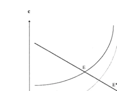
Equation (12) describes the share of aggregate consumption in total output. It shows that a change in g affects c (indirectly) through a change in k, and through a change in the long-run growth rate, n. Equation (13) is the goods market equilibrium condition (GME), and is nothing but equation (11) in per-output terms. Equation (14) is the capital market condition and, finally, equation (15) is derived from the aggregate production function. The equilibrium is depicted in Figure 1 below. The upward-sloping solid locus describing equation (12) is defined for growth rates where the following condition is satisfied: n,
(r2 r), and which simply implies positive and finite consumption to output ratios. The downward-sloping schedule is the goods market equilibrium condition, equation (13), which states that, other things being equal, a lower consumption to output ratio implies a higher investment and, hence, a higher long-run growth rate. Equilibrium is achieved at point E, where the GME schedule intersects with the c˙50 locus. Note also that, unlike the model with decreasing returns, growth never ceases in the present model: the economy always grows at the constant rate, n. This, in turn, implies that there are no transitional dynamics in this model, as consumption jumps to put the economy in equilibrium.
Implications of Finite Horizons
Perhaps, the best way to examine the role of the finite lives assumption is to make a comparison with the infinite horizon case. As is well known, this can be easily done with Blanchard-type consumers, as forl 50 one can get the infinite horizon representative consumer case. In terms of Figure 1, whenl50, the c˙50 locus becomes just a vertical line at point (n5r2r), the point which corresponds to the modified golden rule (MGR). As one can easily see from Figure 1, nl50.nl.0(compare E with E* in Figure 1). The intuition behind this is the following: from equation (6), a lower l implies a lower propensity to consume out of wealth (in terms of Figure 1, a lowerlimplies a shift of the c˙50 locus downwards to become the dot locus, which means a lower consumption ratio and a higher growth rate). As l tends to zero, the propensity to consume (l1 r) goes down and, thus, aggregate consumption goes down too; hence, savings, investment and the long-run growth rate all go up. In other words, (C˙ /C)l50.(C˙ /C)l.0, which implies9 that whenl 50, C tomorrow is bigger than C today, i.e., there is a greater willingness to save today, resulting in a higher growth rate.
IV. The Effects of an Increase in Public Investment
We consider, here, the following fiscal policy experiment. Starting from an initial steady state, the government raises its spending (per unit of output) on infrastructure, financing this by an equal increase in taxes. A close inspection of equations (12)–(15) reveals that they define a system of four equations in four unknowns (k,c,r,n). To start with the effect of g on k, intuitively one would expect that an increase in g would reduce k, because of the complementarity assumption (see, also, equation (15)). An increase in g, financed by
9This consumption externality which leads to a higher consumption ratio and a lower rate of growth in the case ofl.0, is totally different from the inefficiency which arises in the Diamond two-period overlapping generations model. In the latter, oversaving rather than undersaving arises, and this is due to the life-cycle pattern of wage income. In the Diamond (1965) model, wages are positive in the first period and zero in the second; in other words, labor income declines sharply over the life-cycle, whereas with Blanchard-type consumers, labor income is invariant with age. See Jones and Mannuelli (1990) for a recent treatment of the effects of taxation in a two-period OLG model.
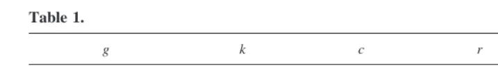
an equal increase in taxes, would also crowd out private consumption, as private wealth (physical capital, k and labor income—see equation (4) and our discussion that follows equation (10) would be reduced. The effects of g on r and n are less straightforward. From equation (14), an increase in g clearly has two opposite effects on r; also, equation (13) shows that an increase in g has two opposite effects on the long-run growth rate: a (direct) negative effect (which can be checked easily from the numerator of equation 13), and two (indirect) positive effects through the reduction in k and c. As a result, theoretically, the effects of government spending on real interest rate, r, and long-run growth rate, n, could be overturned after a point. As it turns out, it is quite difficult to derive these effects analytically. Therefore, we solved the model numerically and, in Table 1 above, we report these comparative statics results (note that the effects of g on k and r can also be algebraically derived).
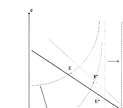
because the rate of consumption goes down by less in the finite horizon case, as people value consumption in the present more highly. More specifically, a permanent increase in g, matched by an increase in present and future taxes, reduces consumption growth by less in the case ofl. 0, as part of the higher future taxes which have to be raised are paid by future (yet unborn) generations. As a result, the growth rate at the (new) steady state is lower in the finite horizons case than in the infinite horizon model (compare point E9
with E** in Figure 2).
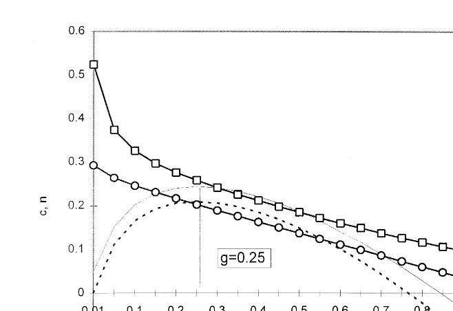
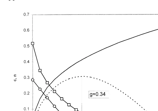
Turning back to Table 1, we see that beyond a certain value of government spending, g*, the growth rate falls with increases in g for reasons mentioned already—namely, that the fall in savings (12g2c) outweighs the rise in the marginal productivity of capital (fall in k). This is well depicted in Figure 3 below (Figure 3 assumes the same parameter values as in Table 1), which shows that public investment is growth-enhancing up to a certain value of government spending to output ratio, g*, which represents the growth-maximizing value of g. Perhaps, not surprisingly— given the identical production struc-ture—the optimal value of g* within our model with finite horizons is equal to the value of g* in the Barro (1990) infinite horizon framework,10corresponding to the productive-efficiency condition, the Barro rule, thatf9 51 [see Barro (1990, pp. S109 –S110)]. The Barro rule states that the optimal provision of government productive services implies that a unit increase in government spending raises output by one unit. If output is raised by less than one unit, government productive services are overprovided ( g . g*), whereas if output is raised by more than one unit, government services are underprovided ( g,g*). With a Cobb-Douglas production function, the Barro rule implies g*5a[Barro, (1990)]; namely, the optimal public investment ratio turns out to be equal to its share in the production function. With finite horizons (and a Cobb-Douglas production function), g* is still given by the Barro rule, as this rule arises directly from the production externality effects, due to public investment rather than from the consumption externality effects arising out of finite horizons (l.0). Note, however, that in contrast to the Barro (1990) infinite horizon framework where, with lump-sum taxes, the growth rate monotonically
10In other words, optimal g* is independent ofl.
rises with increases in g, our simulations suggest that one still obtains the hump-shaped Barro curve (and thus an optimal value for g) even with lump-sum taxes11, because of the finite lives structure. The difference is that the growth-maximizing value of g is higher in the case of lump-sum taxes, relative to g* in the case of output taxes, which is what we would expect (see Figure A.1 in Appendix).
We also performed sensitivity analysis for the most important parameters of the model. It appears that the effects of a rise in g upon consumption, growth, etc., both in the finite lives model and in the infinite horizon model, are quite robust to alternative specifications to the benchmark case of parameter values. Thus, our results are robust to a wide range for the time preference parameter,r(andl), in the range3(0.01, 0.1), and the production side parameter,a3(0.2, 0.6). In particular, g* 5a appears always to be the case for different values of a. In addition, the change in the growth rate (in percentage terms) is larger in the finite horizon case relative to the infinite horizon case. The intuition behind this is along the same lines as in Section III (second subsection), namely that the rate of change in consumption is lower in l. 0 than inl5 0.
We finally turn to welfare considerations. It can be shown that the integral in equation (1) yields:
U5lnv 1ln~l 1 r!2ln~r1l!1r2r
l 1 r. (16)
From equation (16), one can easily derive that (dU/dr) .0, provided thatr,r, which is always the case with finite horizons a` la Blanchard, as only then is the (individual) growth rate of consumption positive (see equation (3)). Using equations (12)–(15), it can
11With a lump-sum tax system, the marginal rate of tax with respect to production is zero. In the absence of a labor/leisure choice, this tax amounts to a consumption tax.
be shown (see, also, Table 1) that r and n move together in the same direction. Hence, maximization of n with respect to g is equivalent to maximization of r with respect to g, which finally is equivalent to maximization of U with respect to g. In other words, with a Cobb-Douglas production function, the growth-maximizing rate of public investment, g, is also the welfare-maximizing rate of g, provided that the above condition (r,r) holds.12
V. Concluding Remarks
This paper examined the effects of government spending on infrastructure within an endogenous growth model populated by consumers within finite horizons. Our framework combined Blanchard-type consumers with Barro-type producers who benefit from pro-ductive government services. Our objective was to highlight the role of finite horizons, and also compare and contrast the effects of government spending within the above framework with those in the infinite horizon representative model. The main results of the paper are as follows: 1) Along the rising part of the Barro curve, a permanent increase in government spending on infrastructure, matched by an increase in present and future income taxes, reduced the consumption share of output by less in the finite horizon case relative to the infinite horizon case, as part of higher future taxes which have to be raised will be paid by future (yet unborn) generations. As a result of this consumption exter-nality, the change in the growth rate was bigger in the finite horizon case relative to the infinite horizon case. The outcome is that the growth rate at the new steady state was lower in the finite horizon case than in the infinite horizon model. 2) A hump-shaped curve (the Barro curve), showing the non-monotonic relationship between government spending on infrastructure and long-run growth, can be obtained in a model with finite horizons even with lump-sum taxes; this is in contrast to the Barro (1990) infinite horizon framework. 3) In a model with finite horizons and a Cobb-Douglas production function, with government services as a factor along with private capital, the growth-maximizing level of government expenditure is also given by the Barro rule. 4) Finally, the paper derived, analytically, a condition under which the growth-maximizing level of public investment maximizes also the utility attained by the representative consumer with finite horizons.
We are grateful to John Driffill, Sugata Ghosh and one Editor of this Journal for useful discussions and suggestions. We especially thank three anonymous referees, as the present version owes a lot to their detailed and constructive comments, and seminar participants at our institutions for helpful feedback. We are responsible, however, for any remaining errors.
References
Aschauer, D. Feb. 1988. The equilibrium approach to fiscal policy. Journal of Money, Credit and
Banking 20:41–62.
Aschauer, D. Mar. 1989. Is public expenditure productive? Journal of Monetary Economics 23:177–200.
Barro, R. Oct. 1990. Government spending in a simple endogenous growth model. Journal of
Political Economy 98:S103–S125.
Barro, R., and Sala-i-Martin, X. Oct. 1992. Public finance in models of economic growth. Review
of Economic Studies 59(4):645–661.
Barro, R. and Sala-i-Martin, X. 1995. Economic Growth. New York: McGraw-Hill.
Baxter, M., and King, R. Jun. 1993. Fiscal policy in general equilibrium. American Economic
Review 83(3):315–334.
Blanchard, O. Apr. 1985. Debt, deficits, and finite horizons. Journal of Political Economy 93(2): 223–247.
Cass, D. Jul. 1965. Optimum growth in an aggregative model of capital accumulation. Review of
Economic Studies 32:233–240.
Cass, D., and Yaari, M. 1967. Individual savings, aggregate capital accumulation and efficient growth. In Essays on the Theory of Optimum Economic Growth (K. Shell, ed.). Cambridge, MA: MIT Press, pp. 117–132.
Diamond, P. Dec. 1965. National debt in a neoclassical growth model. American Economic Review 55(5):1126–1150.
Easterley, W., and Rebelo, S. Dec. 1993. Fiscal policy and economic growth: An empirical investigation. Journal of Monetary Economics 32:389–405.
Futagami, K., Morita, Y., and Shibita, A. 1993. Dynamic analysis of an endogenous growth model with public capital. Scandinavian Journal of Economics 95(4):607–625.
Jones, L., and Rodolfo M. 1990. Finite lifetimes and growth. NBER Working Paper #3469. King, R. and Rebelo, S. Oct. 1990. Public policy and economic growth: Developing neoclassical
implications. Journal of Political Economy 98(5):S126–S150.
Kocherlakota, N., and Kei-Mu, Y. May 1996. A simple time series test of endogenous vs. exogenous growth models: An application to the United States. Review of Economics and Statistics 78(2):126–134.
Kocherlakota, N., and Kei-Mu, Y. 1997. Is there endogenous long-run growth? Evidence from the United States and the United Kingdom. Journal of Money, Credit, and Banking 29:235–262. Rebelo, S. Jun. 1991. Long-run policy analysis and long-run growth. Journal of Political Economy
99(3):500–521.
Romer, P. Oct. 1986. Increasing returns and long-run growth. Journal of Political Economy 94(4):1002–1037.
Saint-Paul, G. Nov. 1992. Fiscal policy in an endogenous growth model. Quarterly Journal of
Economics 107(4):1243–1259.
Solow, R. Feb. 1956. A contribution to the theory of economic growth. Quarterly Journal of
Economics 70(1):65–94.