Kredi risk simulasyonu ve temerrüt oranı / temerrüt halinde kayıp oranının ilişkilendirilmesi

SIMULATION OF CREDIT RISK AND MODELING PD/LGD

LINKAGE

EKREM KILIÇ

104626006

İSTANBUL BİLGİ ÜNİVERSİTESİ

SOSYAL BİLİMLER ENSTİTÜSÜ

FİNANSAL EKONOMİ YÜKSEK LİSANS PROGRAMI

TEZ DANIŞMANI : DOÇ.DR. EGE YAZGAN

2007

ii

Simulation of Credit Risk and Modeling PD/LGD Linkage

Kredi Risk Simulasyonu ve Temerrüt Oranı / Temerrüt Halinde Kayıp

Oranının İlişkilendirilmesi

Ekrem Kılıç

104626006

Doç.Dr. Ege Yazgan :

Yrd.Doç.Dr. Sema Bayraktar :

Arş.Gör.Orhan Erdem :

Tezin Onaylandığı Tarih :

Toplam Sayfa Sayısı:

Anahtar Kelimeler (Türkçe)

Anahtar Kelimeler (İngilizce)

1) Kredi Riski

1) Credit Risk

2) Monte Carlo Simulayonu

2) Monte Carlo Simulation

3) Basel II

3) Basel II

4) RMD

4) VaR

iii

Abstract

Measurement and management of the credit risk has emerged as the one of the most challenging and hottest area of the risk management in financial markets. There are numerous factors motivating that result. The most important motivation of the market is the Basel II Capital Adequacy Accord. Other factors are the increasing number of the defaults all around the world and the rise of the financial derivatives.

In this thesis, I analyzed the simulation of the credit risk and I incorporated PD/LGD linkage to two Credit VaR models (CreditMetrics and CreditRisk+) with a hypothetical portfolio of 500 loans. I compared 3 different level of recovery risk with these 2 models. I found that overlooking PD/LGD correlation leads us to underestimate the credit risk.

Özet

Kredi riskinin ölçülmesi ve yönetilmesi finansal risk yönetiminin en ilgi çekici alanlarından biri haline geldi. Bu sonucu ortaya çıkaran çok sayıda factor var. Fakat, piyasanın bu anlamda en önemli motivasyonu Basel II Sermaye Yeterlilik Uzlaşmasıdır. Diğer önemli faktörler ise, tüm dünyada temerrütlerin artan miktarı ve finansal türev ürünleri kullanımındaki artış olarak sayılabilir.

Bu tezde, 500 krediden oluşan bir hipotetik kredi portfoyü kullanılarak, kredi riskinin simulasyonu analiz edildi ve temerrüt oranı ve temerrüt halinde kayıp oranı arasındaki bağlantı iki Kredi RMD modeline eklendi (CreditMetrics ve CreditRisk+). Temerrüt oranı ve temerrüt halinde kayıp oranı korelasyonunun göz ardı edilmesinin riskin düşük tahmin edilmesine yol açtığı bulundu.

iv

Table of Contents

1 Introduction ... 1

2 Basic Concepts in Credit Risk ... 8

2.1 Probability of Default ... 8

2.1.1 Black-Scholes-Merton Model ... 10

2.1.2 KMV’s Expected Default Frequency (EDF) ... 11

2.1.3 Ratings ... 12

2.1.4 Calibration of Default Probabilities to Ratings ... 13

2.2 Loss Given Default ... 17

2.3 Exposure at Default ... 21

2.4 Expected Loss ... 22

2.5 Unexpected Loss ... 22

3 Credit Risk Models ... 23

3.1 CreditMetrics Model ... 23

3.2 CreditRisk + Model ... 26

3.3 Incorporation of PD/LGD Linkage ... 27

3.3.1 PD/LGD Linkage in CreditMetrics ... 28

3.3.2 PD/LGD Linkage in CreditRisk+ ... 30

4 Simulation and Results ... 32

4.1 Features of the Portfolio ... 32

v

4.3 Monte Carlo Simulation ... 38

4.3.1 Sketch of Monte Carlo Simulation ... 38

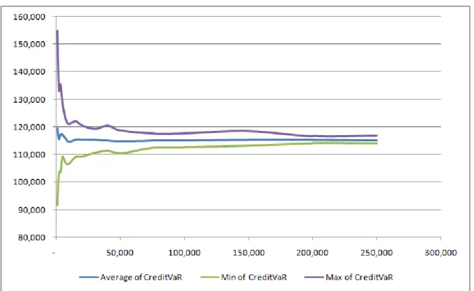
4.3.2 Number of Trials ... 40

4.4 Risk Sensitivities ... 41

4.5 Results ... 42

5 Conclusion ... 49

6 References ... 51

Appendix – Fitting Beta Distribution ... 57

Appendix – Fitting Gamma Distribution ... 57

Appendix – Kernel Density Estimator... 59

vi

List of Tables

Table 1 Definitions of Credit Ratings ... 13

Table 2 Moody's one-year default rates by year and alpha-numeric rating, 1983-1999 15 Table 3 Calibration Result ... 17

Table 4 Moody’s LGD data ... 20

Table 5 Comparison of LGD models with CreditRisk+ ... 42

Table 6 Comparison of LGD models with CreditMetrics ... 43

Table 7 Error due to ignorance of PD/LGD linkage ... 43

Table 8 99.5% CVaR contributions of different risk groups under CreditMetrics with constant LGD ... 60

Table 9 99.5% CVaR contributions of different risk groups under CreditMetrics with stochastic LGD ... 60

Table 10 99.5% CVaR contributions of different risk groups under CreditMetrics with PD/LGD linkage ... 61

Table 11 99.5% CVaR contributions of different risk groups under CreditRisk+ with constant LGD ... 61

Table 12 99.5% CVaR contributions of different risk groups under CreditRisk+ with stochastic LGD ... 62

Table 13 99.5% CVaR contributions of different risk groups under CreditRisk+ with PD/LGD linkage ... 62

vii

List of Figures

Figure 1 The default rate for Black-Scholes-Merton model... 11

Figure 2 Moody's One-Year Default Rates Between 1983-1999 ... 16

Figure 3 Calibrated PD Graph ... 16

Figure 4 Calibrated PD St.Dev. ... 17

Figure 5 Probability of default and exposures of loans in the portfolio ... 33

Figure 6 Loss given default and exposure of loans in the portfolio ... 33

Figure 7 Rating and collateral distribution of the portfolio ... 34

Figure 8 Exposure concentration at each PD/LGD pair ... 35

Figure 9 CVaR% of CreditMetrics and CreditRisk+ with static LGD model at different levels of default correlation ... 38

Figure 10 Average of CVaR and its range with different number of trials. ... 40

Figure 11 Tail of loss distribution under different LGD models of CreditRisk+ ... 44

Figure 12 Tail of loss distribution under different LGD models of CreditMetrics ... 45

Figure 13 Comparison of CreditMetrics and CreditRisk+ at obligor level ... 46

Figure 14 Comparison of 99.5% CVaR of constant LGD and stochastic LGD models with CreditMetrics ... 47

Figure 15 Comparison of 99.5% CVaR of constant LGD and PD/LGD linked models with CreditMetrics ... 48

Figure 16 Sensitivity of models to PD/LGD correlation ... 49

Figure 17 Shapes of different beta distributions fitted to collateral types ... 57

viii

List of Abbreviations

CVAR – Credit Value at Risk EAD – Exposure at Default ECAP – Economic Capital EL – Expected Loss

LGD – Loss Given Default PD – Probability of Default UL – Unexpected Loss

1

1

Introduction

Measurement and management of the credit risk has emerged as the one of the most challenging and hottest area of the risk management in financial markets. This notable and increased focus on credit risk has been initiated by the concerns of regulatory authorities, risk measurement necessities of financial institutions bearing loan portfolios and investors who are willing to trade these risks.

From regulatory point of view, the credit risk has been emplaced at the center of the capital requirement system starting from the first Accord of Basel Committee on Banking Supervision. Basel I which aims “to strengthen the soundness and stability of the international banking system” (Basel Committee on Banking Supervision, 1988) was an important start for an international capital standard, and it set capital adequacy rules for banks. This first attempt was largely successful but developments in the market accentuated certain limitations in the Accord, creating the necessity for revisions to the Accord. The first attempt to improve the Basel I was 1996 Amendment. With this amendment, the banks allowed to use internal models for their trading books. After 1996 Amendment, regulatory rules for trading books and for the calculation of the market risk have matured. However 1996 Amendment brought no improvement related with the credit risk, it remained as a weakness of the Accord. The main weakness of the Basel I in credit risk context is broadness of the imposed weightings. This weakness creates several problems. First, risk sensitivity of the required capital is very limited. For instance, let us assume that the bank has two loans; one to a recently started firm and the other to one of the biggest firms in the country. In this case Basel I requires exactly the same capital for both loans. Secondly, no default correlation allowed in this calculation. Therefore, the very basic risk management rule of diversification has no effect on the required capital. If the

2

bank has only one big loan is treated same as if it would have thousand small loans. Finally, since the weights are constant over time, they do not reflect the cyclicality of the credit risk. However, Fama (1986) and Wilson (1997) find that cyclical features in the probability of default, especially in the case of recessions when defaults increase dramatically. Bangia, Diebold and Schuermann (2000) and Nickell, Perraudin and Varotto (2000) analyzed macroeconomic and industrial effects on ratings downgrades and defaults, and find that they are more likely to occur during downturns of business cycle.

To address the weaknesses in the Basel I accord, committee published International Convergence of Capital Measurement and Capital Standards, a Revised Framework, (commonly known as Basel II), in June 2004. The principal aim of the Basel II is to improve the risk sensitivity of capital allocation. Basel II based on three pillars; minimum capital requirements, supervisory committee and market discipline. Pillar 1 of new Accord aims to improve 1988 Accord’s guidelines. The accord provides three options for calculation of required capital for credit risk. Standardized, Foundation Internal Rating Based model and Advanced Internal Rating Based Models from simplified to sophisticated. All of these options provide a more risk sensitive calculation of required capital than the first Accord.

Parallel to regulatory efforts, financial institutions searched for the ways of effective risk management. The studies in this field back to 1970’s, however in last two decades the number of studies increased and methods improved tremendously. We may divide credit risk models into several categories. The first category is based on the framework developed by Merton (1974) called as structural form models. In this framework, the event of default is determined by the level of the firms’ assets. If the market value of the assets of the firm is lower than it liabilities, default occurs. Therefore, the loan payment is always the

3

minimum of the debt or market value of the assets. Under this model, all credit risk components, including default and the recovery rate, are directly linked to the financial structure of the firm, with using asset volatility and the leverage. Thereby recovery rates are endogenous variables under structural form models. Another feature of these models is probability of default and recovery rates tend to be inversely related. For instance as firm’s value increases, then its probability of default will decrease, on the other hand recovery rate of the firm increases or vice versa.

Recent models adopting the Merton’s framework, removes one unrealistic assumption of Merton’s model that the event of default may only occur at the maturity of the debt. In the original frame work Merton replicates the cash flow structure of a loan with a zero bond and put option. This assumption makes the put option a European type put option and best known Black-Scholes formula becomes applicable. Geske (1977, 1979) considered the debt structure of the firm as a coupon bond in which each coupon payment is viewed as a compound option and a possible cause of default. Other models, called first passage models, instead of using this assumption, allowed the default to occur any point of time between issuance and maturity. Under the first passage frame work, the default may occur when the asset level reaches a threshold during the life of the loan. Some of the recent structural form models provided by Kim et al. (1993), Nielsen et al. (1993), Longstaff and Schwartz (1995), Hull and White (1995).

The assumption of flat and fixed term structure of interest rates is another source of criticism on the Merton’s model. Jones et al. (1984) claimed that “there exists evidence that introducing stochastic interest rates, as well as taxes, would improve the model’s performance.” Usage of stochastic interest rate models allowed to introduce correlation between the firm’s asset value and the short rate, and have been considered, among others,

4

by Ronn and Verma (1986), Kim et al. (1993), Nielsen et al. (1993), Longstaff and Schwartz (1995).

Another category of credit risk models, attempted to adress the shortcomings of the structural form models called as reduced form models. The main difference between the structural form models and reduced form models is that the former provide the link between the probability of default and the financial variables of the firm. Reduced form models, on the other hand, extract the probability of the default from market prices of the defaultable instruments of the firms. Moreover reduced form models assumed seperate dynamics for probability of default and recovery rates. As a result reduced form models based on exogenous recovery rates and recovery rates and the default probability are independent. In other words, in structural models, due to the assumption of complete information, investors are able to predict the arrival of default. This predictability of default implies zero short-term credit spreads for the firm’s debt, which is not consistent with the short-term spreads seen in practice. Reduced form models overcome this limitation specifying an exogenous default intensity which makes default an unpredictable event. Both probability of default and recovery rate may vary stochastically. Some studies introducing reduced form models are Litterman and Iben (1991), Madan and Unal (1995), Jarrow and Turnbull (1995), Jarrow et al. (1997), Lando (1998), Duffie and Singleton (1999), Duffie and Lando (2001), Çetin et al. (2004), Giesecke (2004, 2005), Giesecke and Goldberg (2004).

For credit risk analysis of loan portfolios Credit VaR models provide a clear methodology for the banks. Credit VaR models aimed at measuring the potential loss with a predetermined confidence level that a portfolio could suffer during a specified time horizon (generally on year). Some of these Credit VaR models are based on the

5

assumptions of the structured form models like JP Morgan’s CreditMetrics (Gupton et al, 1997) and KMV’s CreditPortfolioManager, while some others are based on reduced form models like Credit Suisse Financial Products’ (1997) CreditRisk+ and McKinsey’s CreditPortfolioView (Wilson, 1997). The main output of all Credit VaR models is the probability density function of the future losses on a loan portfolio. Generating this density function, the financial institute can calculate its expected loss and economic capital which is a cushion for unexpected losses.

In single loan level, credit risk has three main ingredients; exposure at default, the probability of default and the loss given default. In the portfolio level, default correlation and rating migrations are also important components. A recent area of modeling is the linkage between the probability of default and the loss given default. The main idea behind that is when the economy goes into a recession as probability of defaults rise, the loss given default also increases. Several studies empirically supported the idea. In this study, I will also consider the PD/LGD correlation. The studies considers PD/LGD linkage includes, Frye (2000), Jarrow (2001), Carey and Gordy (2003), Bakshi et al (2001), Altman et al (2001, 2005), Acharya et al (2003) and Gupton and Stein (2005).

The model suggested by Frye (2000) extends the approach proposed by Finger (1999) and Gordy (2000) to probability of default and loss given default correlation. In these models default is driven by a single systematic factor which affects all obligors and idiosyncratic factor which is unique to each obligor. Frye’s model assumes that the systematic factor that representing the state of the economical environment, affects the amount of loss at the event of default. Therefore when the economy is good, the number of defaults decline and the recovery at default increases. On the other hand, if the economy is in a down-turn, the number of defaults increases and the recovery at default decrease. The

6

intuition behind Frye’s framework is based on the value of the collaterals. The value of the collaterals depend on the economic conditions as other asset of the firms, therefore in the times of financial distress due to economic conditions, collaterals’ value will decline. This implies a positive correlation between loss given default and conditional default probability. To incorporate this effect, Frye links both probability of default and the loss given default to the systematic factor by imposing a single factor model for loss given default similar to default event. The correlation between default and loss given default results from this mutual dependence.

Using Moody’s Default Risk Service Database from 1983 to 2001, Frye (2005) empirically find that loss given default rise as default rates. But at the same time the risk is higher for lower loss given default groups. In addition to this, Frye claims that the loss given default sensitivity increases the loss in high default periods.

Using defaulted bond data Altman et al (2005) find empirical results consistent with Frye’s intuition. However they also find that econometric univariate and multivariate models may explain an important portion of the variance of the bonds loss given defaults. Therefore they conclude single systematic risk factor is less predictive than Frye’s model suggest.

Altman et al (2005) examined the implications of the PD/LGD linkage to credit risk modeling. They used the setup of CreditRisk+ of CSFB and extended the model to include PD/LGD linkage. They used Monte Carlo simulations to compare the differences between key risk parameters with respect to loss given default setup in the model. They compared static, stochastic and correlated stochastic loss given default models. They showed that both expected loss and unexpected loss is underestimated without including PD/LGD correlation.

7

In this theses I examine the same effect implementing PD/LGD linkage of Frye (2000) to both CreditMetrics and CreditRisk +. I compare the results between credit risk models and between LGD models. Calculating the Credit VaR contributions of each loan, I analyze the effect of credit size, credit quality and collateral on the differences.

The contribution of the paper is in four aspects. First, I compared the effects of PD/LGD correlation with two models. Second, I calibrated numerical version of CreditRisk+ (which implemented similar to Altman et al (2005)) to CreditMetrics. Thirdly, I extent CreditRisk+ implementation of Altman et al (2005) by introducing a random which represents the idiosyncratic risk of collateral part as in Frye (1999). This also make possible to compare both models. Finally, I examined the results not only portfolio level but also single loans level, and analyzed the effect of PD/LGD correlation on different risk characteristics.

The analysis showed that ignorance of PD/LGD linkage, underestimates the risk related with the recovery risk. In addition to this, it is shown that usage of stochastic LGD is inadequate to cover the recovery risk.

Outline of the following sections is as follows. First basic concepts in Credit Risk are described briefly. Secondly, credit risk models in this thesis and incorporation of PD/LGD linkage to these models are explained. Thirdly, I discuss assumptions of the simulation and results of the models. Finally I conclude.

8

2

Basic Concepts in Credit Risk

2.1

Probability of Default

The key element of credit risk is default risk which can be defined as the uncertainty regarding an obligor’s ability and willingness to service its debt obligations. And the common measure of default risk is the probability of default. Modeling and quantifying default probability is a very difficult task. First of all, default event is highly rare, therefore most of the time; the data for analysis are very limited. Second, although the general level of the default probabilities across different loans determined by the general economic environment, the default rate estimation of an obligor is based on the factors directly related with the obligor. And most of time determination of the credit grade of an obligor is highly subjective procedure which may change with respect to the expectations of the rating agency on the sector, economy, firms’ plans etc... In this section we will discuss different approaches for estimation of default probabilities.

As I mentioned before, assigning the default probabilities of each obligor in the loan portfolio is not an easy task. To do this task one may follow mainly two different approaches. One way for estimating default probabilities is the usage of market data. This approach is basically based on the credit spreads of traded products bearing credit risk such as corporate bonds and credit derivatives. Second way of estimation for default probabilities uses the ratings systems. In this approach, default probabilities are associated with rating classes and ratings are assigned to customers either by external rating agencies or by bank’s internal rating system. Because it is not always possible to find necessary market data, the second approach is much more useful for modeling a large credit portfolio. Especially in emerging, only few corporate bonds might be available, and there may be no default data related with these corporate bonds. In addition to this, even if there

9

is mature market for defaultable bonds, the products in the market may not provide necessary information for all loans in the portfolio. Hence, most of the credit risk models are based on rating systems. From this point of view the measure of default probability of a firm or sovereign is the average frequency of the obligors which were in the same credit grade. However, the usage of these or similar average default rates are criticized for several reasons, Duffie and Singleton (2003) mentions three key issues;

 Since credit rating is a subjective opinion, the degree of consideration related with subjective factors is not comparable. One important consequence of this appear considering the extent of losses at default and other aspects of anticipated performance for investors over life of the debt. The degree of this kind of subjective factors may change over time and among rating agencies.  Credit ratings are measure of relative credit quality, therefore they are more

stable through business cycles than they supposed to be.

 Averages are stationary measures of default probability; therefore they are inadequate to reflect the dynamics of market or the firm. Recent events or new information about the firm does not affect the rating immediately. Commonly respect to the degree of the importance of the news the rating agency may revise the firm’s rating. However, this might take time, because they may repeat all rating process. Moreover, if the rating agency does not consider the information as important as to revise rating, it may ignore the new information, and leave the rating as it is.

In this thesis I used Moody’s data for probability of default and calibrated as I explain later. Before that, I will review the other models.

10

2.1.1 Black-Scholes-Merton Model

In this approach the loan considered as a zero bond which matures at time 𝑇 and its face value is equal to 𝐷. As it was explained in the previous section, the model assumes that default can only occur at the maturity, the condition for default is 𝐴_𝑡 ≤ 𝐷 ; where 𝐴_𝑡 is the market value of the firm’s assets at time 𝑇 .

Assuming log-normal asset prices, the distance to default derived as;

𝑋_𝑡 =ln 𝐴𝑡 −ln 𝐷 𝜎

Then, under this model, the probability of default occurring at the maturity is;

𝑃 = 𝑁 −𝑢 𝑡, 𝑇

where 𝑁(. ) is the probability density function of normal distribution and

𝑢 𝑡, 𝑇 =𝑋𝑡+ (𝜇 − 𝛾 − 𝜎2/2)/𝜎 𝑇 − 𝑡

In this formula (𝜇 − 𝛾 − 𝜎2/2)/𝜎 represents the rate of change of the mean distance to default and 𝑢 𝑡, 𝑇 is the number of standard deviations that 𝑋_𝑡 exceeds the mean distance to default (𝜇 is the mean rate of return on assets and 𝛾 is the payout rate and 𝜎 is asset volatility).

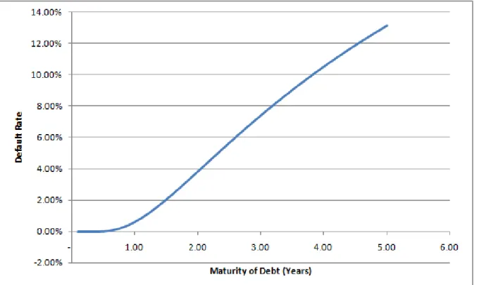
For example let us consider a firm withμ−γ= 15% σ= 10%, A_t = 100 and D =

90, the probability of default for T − t = 1 is 0.61%. Figure 1 shows how default probability changes as the maturity of the debt changes. As it can be seen, the longer maturity means higher default probability, because as time path gets longer the uncertainty increases. If we decrease the debt to 80, probability falls to 0.01%, it shows that the model highly sensitive to the level of the debt.

11

Figure 1 The default rate for Black-Scholes-Merton model

2.1.2 KMV’s Expected Default Frequency (EDF)

KMV Corporation developed their popular EDF measure which is based theoretical framework of Black-Scholes-Merton model.

First KMV has observed from its huge default database that firms are more likely to default when their asset size reached a level between their short term debts and the long term debts. Therefore they switch the threshold level D with the default point that is defined as;

𝐷𝑃𝑇 = 𝐷_{𝑠𝑕𝑜𝑟𝑡} + 0.5 ∗ 𝐷_{𝑙𝑜𝑛𝑔}

They also define an index, called distance to default, DD as follows;

DD = E AT − DPT

12

where E A_T is the expected value of firm’s assets market value at time T and σ is the standard deviation of A_T.

Rather than using Black-Scholes-Merton formula for default probability, KMV estimate the frequency of the default with which firms of a given 1-year expected distance to default have actually defaulted before. By doing that, KMV calibrates the theoretical distance to default with historical default data base and creates a mapping between distance to default and EDF. In addition, KMV calculates the asset volatilities from equity volatilities recognizing the effect of current leverage of the firm to the asset volatility.

2.1.3 Ratings

Basically ratings are the opinion of the rating agency on the credit worthiness of an obligor. Hereby, both qualitative and quantitative data are used for analysis. Since rating is an opinion, in practice it is mainly based on experience and the judgment of the credit analyst rather than a pure mathematical procedure based on the historical data.

Credit rating may be provided by external credit rating agencies e.g. S&P, Moody’s and Fitch. It may also be provided by the bank’s internal rating model, but of course in this case, bank need to invest more in their system. During the analysis of the customers’ creditworthiness some important factors indicating the future financial strength are the followings;

 Future earnings and cash flow

 Debt and debt structure (maturity, type etc.)  Capital structure

 Liquidity of the assets  Analysis of conjuncture

13

 Analysis of the sector

 Management quality and corporate governance

Table 1 Definitions of Credit Ratings

Credit rating agencies uses an ordered scale of ratings in terms of letter system describing the credit worthiness of the borrower or issuer. Letter systems of S&P and Moody’s are different but they can easily be mapped as in the Table 1. Behind the letter system given in the Table 1, rating agencies are using a finer scale for a more accurate distinction between different qualities.

2.1.4 Calibration of Default Probabilities to Ratings

Assigning default probabilities to the rating classes is called as calibration. In this section, I will mention the basics of this calibration. At the end of the calibration process, we will end up with a mapping between rating classes and default probabilities as follows;

Moody's S&P Fitch Definition

Aaa AAA AAA Highest quality; extraordinary ability to repay principal and interest

Aa AA AA High quality; very strong capacity to repay A A A Upper medium grade; strong capacity to

repay

Baa BBB BBB Medium grade; adequate capacity to repay

Ba BB BB Speculative; repayment protection

moderate

B B B Highly speculative; lightly protected Caa CCC CCC Of poor standing; possibility of default Ca CC CC Minimally protected; default probable

C C C In actual or imminent default

14

𝐴𝐴𝐴, 𝐴𝐴, 𝐴, … , 𝐶 → [0,1]

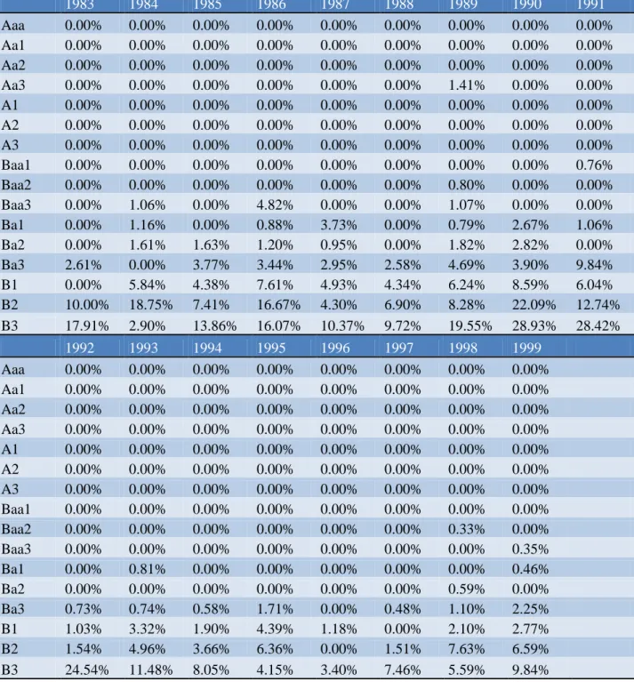
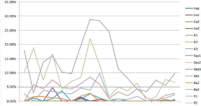
In this thesis I will explain the calibration process by means of Moody’s public data(Keenan, Hamilton, & Berthault, 2000). In Moody’s data Exhibit 29 shows the one year default probabilities of finer ratings of Moody’s from 1983 to 1999.

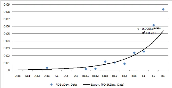
As it is shown in Table 2, the Moody’s data, an important observation is that for the top credit ratings there is no default observed. One should not be surprised that most of the times top rating classes are lack of default history or they have no default history at all. Even there is no default history at all, it would not be appropriate to take the historical zero default rate as the model parameter for the credit risk calculations. Therefore we need to assign small but positive default rates for these rating classes. For doing this, I will calibrate probability of default values. The calibration procedure contains of two stage; for each rating class, I first calculate mean and standard deviation of PD’s. In the second step fit the following regression;

𝑃𝐷 𝑥 = 𝑎 ∗ 𝑒𝑏𝑥

where 𝑎 and 𝑏 coefficients of the regression and 𝑥 is an integer indicating the rating level (1 for Aaa and 16 for B3).

Taking the logarithm of the equation, the regression can be estimated by using ordinary least squares. This regression is estimated for both PD and standard deviation of PD. The results are shown in Table 3 Calibration Result. In this thesis, calibrated PD will be used.

15 1983 1984 1985 1986 1987 1988 1989 1990 1991 Aaa 0.00% 0.00% 0.00% 0.00% 0.00% 0.00% 0.00% 0.00% 0.00% Aa1 0.00% 0.00% 0.00% 0.00% 0.00% 0.00% 0.00% 0.00% 0.00% Aa2 0.00% 0.00% 0.00% 0.00% 0.00% 0.00% 0.00% 0.00% 0.00% Aa3 0.00% 0.00% 0.00% 0.00% 0.00% 0.00% 1.41% 0.00% 0.00% A1 0.00% 0.00% 0.00% 0.00% 0.00% 0.00% 0.00% 0.00% 0.00% A2 0.00% 0.00% 0.00% 0.00% 0.00% 0.00% 0.00% 0.00% 0.00% A3 0.00% 0.00% 0.00% 0.00% 0.00% 0.00% 0.00% 0.00% 0.00% Baa1 0.00% 0.00% 0.00% 0.00% 0.00% 0.00% 0.00% 0.00% 0.76% Baa2 0.00% 0.00% 0.00% 0.00% 0.00% 0.00% 0.80% 0.00% 0.00% Baa3 0.00% 1.06% 0.00% 4.82% 0.00% 0.00% 1.07% 0.00% 0.00% Ba1 0.00% 1.16% 0.00% 0.88% 3.73% 0.00% 0.79% 2.67% 1.06% Ba2 0.00% 1.61% 1.63% 1.20% 0.95% 0.00% 1.82% 2.82% 0.00% Ba3 2.61% 0.00% 3.77% 3.44% 2.95% 2.58% 4.69% 3.90% 9.84% B1 0.00% 5.84% 4.38% 7.61% 4.93% 4.34% 6.24% 8.59% 6.04% B2 10.00% 18.75% 7.41% 16.67% 4.30% 6.90% 8.28% 22.09% 12.74% B3 17.91% 2.90% 13.86% 16.07% 10.37% 9.72% 19.55% 28.93% 28.42% 1992 1993 1994 1995 1996 1997 1998 1999 Aaa 0.00% 0.00% 0.00% 0.00% 0.00% 0.00% 0.00% 0.00% Aa1 0.00% 0.00% 0.00% 0.00% 0.00% 0.00% 0.00% 0.00% Aa2 0.00% 0.00% 0.00% 0.00% 0.00% 0.00% 0.00% 0.00% Aa3 0.00% 0.00% 0.00% 0.00% 0.00% 0.00% 0.00% 0.00% A1 0.00% 0.00% 0.00% 0.00% 0.00% 0.00% 0.00% 0.00% A2 0.00% 0.00% 0.00% 0.00% 0.00% 0.00% 0.00% 0.00% A3 0.00% 0.00% 0.00% 0.00% 0.00% 0.00% 0.00% 0.00% Baa1 0.00% 0.00% 0.00% 0.00% 0.00% 0.00% 0.00% 0.00% Baa2 0.00% 0.00% 0.00% 0.00% 0.00% 0.00% 0.33% 0.00% Baa3 0.00% 0.00% 0.00% 0.00% 0.00% 0.00% 0.00% 0.35% Ba1 0.00% 0.81% 0.00% 0.00% 0.00% 0.00% 0.00% 0.46% Ba2 0.00% 0.00% 0.00% 0.00% 0.00% 0.00% 0.59% 0.00% Ba3 0.73% 0.74% 0.58% 1.71% 0.00% 0.48% 1.10% 2.25% B1 1.03% 3.32% 1.90% 4.39% 1.18% 0.00% 2.10% 2.77% B2 1.54% 4.96% 3.66% 6.36% 0.00% 1.51% 7.63% 6.59% B3 24.54% 11.48% 8.05% 4.15% 3.40% 7.46% 5.59% 9.84%

16

Figure 2 Moody's One-Year Default Rates Between 1983-1999

17

Figure 4 Calibrated PD St.Dev.

Rating Class PD PD St.Dev.

Aaa 0.00% 0.04% Aa1 0.01% 0.06% Aa2 0.01% 0.08% Aa3 0.02% 0.12% A1 0.03% 0.16% A2 0.05% 0.22% A3 0.09% 0.30% Baa1 0.14% 0.42% Baa2 0.24% 0.58% Baa3 0.40% 0.79% Ba1 0.66% 1.09% Ba2 1.10% 1.50% Ba3 1.84% 2.07% B1 3.07% 2.85% B2 5.13% 3.93% B3 8.56% 5.41%

Table 3 Calibration Result

2.2

Loss Given Default

The Loss Given Default (LGD) of a transaction is more or less determined by “1 minus recovery rate”. Therefore the LGD is the portion of the loan that will be lost in the case of default. When the default event occurs, the loss given default includes three types of

18

losses; the loss of the principal, the carrying out costs of non-performing loans, workout expenses.

In practice there are three different approaches to calculate loss given default. First approach uses the market data of defaulted loan soon after the default event. Since the model is based on the loans or bonds that trade in the market, the prices of these assets are directly observable. In this model the price of the defaultable asset just after the default event, is translated into recovery rates. For example, for a par value of 100, if the price of the asset after the default is 45, then recovery rate is 45% and loss given default is 55%. The advantage of this model, the results of the model does not have model error; instead it reflects the market price. Disadvantage of the model, on the other hand, is that for a loan portfolio, probably only few of the loans will be tradable.

The second approach is more complicated than the first approach and needs more detailed data of the defaulted loan. In this approach after the default event occurred, all cash flows of the defaulted loan should be recorded. These cash flows include recoveries from collaterals, extra payments and costs due to legal procedures or liquidation of the assets of the obligor. Collecting theses records, at the end, the bank will get arrays of cash flows for each defaulted loans. The next step is to discount each those cash flows with a proper discount rate. However, determination of the discount rate for the cash flows of a defaulted loan is not obvious. In other words there is no clear methodology for setting the risk premium of a cash flow coming from an asset whose risk has already realized. In this context the types and structure of the collateral should be considered. As an extreme example, the obligor might have cash collateral, therefore the cash flow from this collateral certain. Another example can be a commercial mortgage, independently from the obligor, the risk of the cash flow from the real estate directly determined by real estate itself (expert

19

values for this cases requires consideration). Therefore in determination of the discount rate, one should prefer discount rates with respect to the type of the asset that will be liquidated.

After following the above procedure, the bank calculates single of realized losses given default for each defaulted loan in the portfolio. In the next step these realized loss given defaults should be combined to get a loss given default estimate for the portfolio of loans. Commonly three different averaging approaches can be followed. The first approach is the “dollar weighted” averaging of the realized loss given defaults which can be formulized as;

𝐿𝐺𝐷_𝑝 = 𝐿𝐺𝐷𝑖 ∗ 𝐸𝐴𝐷𝑖

𝑛 𝑖=0

𝐸𝐴𝐷_𝑖

where 𝐿𝐺𝐷_𝑖 is the realized loss given default for the ith defaulted loan, n the number of defaulted loans in the analysis period and 𝐸𝐴𝐷_𝑖 is the exposure of the ith loan. The second approach for averaging realized loss given defaults is simple average. In this approach the portfolio estimate of the loss given default is simple average of single realized loss given defaults. This approach is called as “default weighted” average. And the last approach is the time weighted average of loss given defaults. This approach can be implemented on either default weighted or dollar weighted yearly averages of loss given default. In this approach last year’s average gets the biggest weight, the year before the last year gets the second biggest and so on… However the last approach increases the smoothness of the loss given default and it causes to underestimate the risk when the recently occurred realized loss given defaults are higher. Time averaging also smooth outs the correlation between probability of default and loss given default.

20

Another important point related with the calculation of loss given default for a portfolio is the treatment of the 0% LGD’s. In practice, due to over collateralization, all of the loss can be recovered from the loan, but it should be considered as outliers1.

The last approach for calculation of loss given default is to look at credit spreads on the defaulted risky bonds (i.e. corporate bonds, eurobonds). The risk premiums of non-defaulted risk bonds reflect the expected loss of the bond. Hence, the risk premium contains information about probability of default, loss given default and the liquidity risk. The models using this approach recently developed, these models separate two parameters of credit risk; probability of default and loss given default. One example for this approach is provided Unal et al (2003). They suggest the “adjusted relative spread”, captures risk-neutral recovery information in debt prices and also interest rates. They also find that the recovery rates obtained by this model will be systematically below the actual recovery rates.

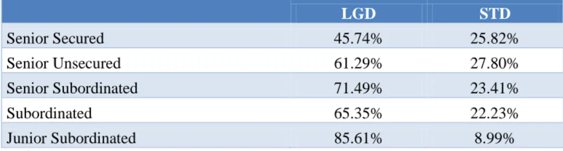
In this thesis I used the LGD data of Moody’s from 1970-2003 as it is presented in Schuermann (2005). The rates are shown .

LGD STD Senior Secured 45.74% 25.82% Senior Unsecured 61.29% 27.80% Senior Subordinated 71.49% 23.41% Subordinated 65.35% 22.23% Junior Subordinated 85.61% 8.99%

Table 4 Moody’s LGD data

1

For Turkey, in practice, number of 0% LGD is not ignorable; therefore instead of using a simple LGD estimate for a group of loans, a proper risk management system should consider the collateral structure of each loan and calculate unique LGD’s for the given collateral structure. To be able to do this, calculation of realized cash conversion rates of each collateral type becomes important. Cash conversion rate can be defined as the ratio of present value of dollar recovery from collateral to collateral’s expert value of collateral. Another issue is the complex collateral structures among loans. Because the collateral structure among loans may be quite different, grouping loans under several collateral structure groups for using average LGD’s may be quite difficult and quite overlooking approach. Considering collateral structure for each loan can be remedy for this problem too.

21

2.3

Exposure at Default

Exposure at Default (EAD) is the total exposure that the bank does have to its obligor. For a term loan determination of EAD is certain, however this is not straightforward for the credit products like lines of credits where an obligor is able to draw extra loan up to a committed limit. Therefore, EAD has two components; the outstanding and the commitment. The outstanding is the loan that the borrower already drawn. In the case of the default the bank is exposed to the total amount of outstanding. The other source of the exposure is the undrawn portion of the commitments and until the time of default the obligor might have extended its loan up to the commitment or somewhere between commitment and current level. Thus, at default the bank is exposed to some portion of unused commitments. Historical default experience shows that most of the time obligors tend to drawn credit lines in the times of financial distress.

Basel II also considers that effect, in Basel II’s foundation IRB method, for example, the EAD for irrevocable undrawn commitments is 75%. In advanced IRB, however, the bank may estimate its own EAD. Estimate of propensity to use undrawn commitments before default should be differentiated across different rating classes and loan types. After defining EAD groups, one can compare the average usage of non-defaulted loans and usage of defaulted loan within group and calculate an estimate for extension of defaulted loans in undrawn commitments. Using the data of Citibank’s large corporate loans from 1988-1993 Asarnow and Marker (1995) empirically analyzed the average revolver utilization of non-defaulted and defaulted loans. They showed that average revolver utilization of defaulted loans is higher than non-default loans in every rating class. Further they found that higher classes use their line less than lower class. In a recent study, using the data of Spanish Credit Register, Jiménez et al (2007) examined corporate credit line usage. They found that the firms using credit lines extensively eventually defaulted on

22

these lines. They also found that credit line default is the dominant explanatory factor for credit line usage.

2.4

Expected Loss

The basic idea of the insurance firms is that pooling several customers with in a basket and distributing the sum of costs related with all customers to the basket. For example in health insurance the cost of few sick customers are covered by the fees of the all customers. Therefore, when the insurance company determines the fee for a group of customers, it considers the expected cost of a customer having the same characteristics with this particular group of clients.

The problem for the bank is exactly the same. To be able to charge correct risk premium banks should examine each obligor. Summing up all risk premiums, bank creates a capital cushion for protecting itself against defaults.

Expected loss of a specific loan is determined by three components; PD, LGD and EAD. Therefore the bank assigns a PD to each obligor, and finds the appropriate LGD level with respect to its collateral and seniority. After analyzing the EAD as it is described in the section2.3, the expected loss of an obligor can be calculated as follows;

L = D ∗ LGD ∗ EAD where D = 1 if default occurs 0 otherwise E L = PD ∗ LGD ∗ EAD

2.5

Unexpected Loss

In section 2.4 I introduced EL as capital cushion for the bank. But holding a capital cushion against expected losses is not adequate. Since EL is just an average, bank should consider the possibility that the real losses might exceed the average. Therefore, in addition

23

to EL reserve, banks should also reserve money for coverage of unexpected losses. This capital is called as economic capital and can be defined as a given percentile of loss distribution (i.e. 99.7%) minus expected loss.

Unexpected Loss (UL) is defined as a measure of the magnitude of deviation of losses from the EL, or in other words the standard deviation of the losses. UL can be defined as the follows;

UL = var L = var PD ∗ LGD ∗ EAD

If we assume that LGD and PD are independent, the unexpected loss becomes;

UL = EAD ∗ var LGD ∗ PD ∗ LGD2 _{∗ PD ∗ (1 − PD)}

In this definition, we look at the credit risk of a single facility; however the banks have to manage credit risk of a portfolio of loans. Another weakness of this definition is that it assumes PD/LGD independency. Note that zero correlation between severity and the default event is not realistic. In fact, recent studies show that bad economic conditions increases both probability of default and the losses.

3

Credit Risk Models

3.1

CreditMetrics Model

The framework of the CreditMetrics is mainly based on the joint default probability of the pair of assets. The joint probability of the assets can be shown for two credit as follows;

𝑝₁₂ = 𝜑(𝑁−1 _𝑝

24

where 𝜑 denotes the cumulative bivariate normal density function, and 𝑝₁ and 𝑝₂are the probability of default of first and second loans respectively. However if we generalize the case to n loan portfolio, we need to use multivariate cumulative normal density function;

𝑝_12…𝑛 = 𝜑(𝑁−1 _𝑝

1 , 𝑁−1 𝑝2 , … , 𝑁−1(𝑝𝑛); 𝜌)

The latter formula requires estimation of the asset return correlation among all pairs of assets. The asset returns can be calculated using observable equity returns. At this point, we are using the equity returns as a proxy for the asset returns, therefore main drawback of the model is how good the equity returns can mimic the asset returns and also how good the asset correlations can be represented by the equity correlations. Although the approach has this drawback, practically it is more accurate than using fixed correlation and is based on data that are more readily available than credit spreads or actual rating changes.

For a real loan portfolio, producing a correlation for each pair of obligors is inefficient. There are two reason for that; scarcity of the data for some obligors and the size of the resulting correlation matrix. Therefore CreditMetrics uses a mapping scheme between obligors and a number of indices. After each obligor mapped to the indices, correlation between obligors are analyzed indirectly incorporating the correlation between indices.

For representing the asset return of a single obligor, CreditMetrics uses the following;

𝑟 = 𝑤₀𝑟₀+ 𝑤₁𝑟₁+ ⋯ + 𝑤_𝑛𝑟_𝑛

where 𝑟 is the normalized asset return and normally distributed with zero mean and unit variance, 𝑟₀ specific risk and the other r’s are the normalized asset returns of the sector indices and they are also normally distributed with zero mean and unit variance. The random factor 𝑟0 is uncorrelated with other factors (𝑟1, 𝑟2, … , 𝑟𝑛).

25

In this representation of the asset return 𝑤₀𝑟₀ called as idiosyncratic part, showing the asset return changes that cannot be related with sectorial effects and represents the risks specific to the obligor. The rest of the formula called as systemic part and represents the sectorial and macro effects on the obligor’s asset return.

The obligor specific risk is a given parameter for this model and can be calculated as follows;

𝜗 = 1 − 1 − 𝑤₀2

where 𝜗 is the obligor specific risk. Using this formula we can find that;

𝑤₀ = 𝜗(2 − 𝜗)

Other weights (𝑤1, 𝑤2, … , 𝑤𝑛) are related with the sectorial mapping of the obligor, and asset volatility of mapped indices. The equation for the remaining factors is the following;

𝑤_𝑖 = 𝛼𝑖𝜎𝑖

𝑛𝑖,𝑗 =1𝛼𝑖𝛼𝑗𝜎𝑖𝜎𝑗𝜌𝑖𝑗

∗ (1 − 𝜗)

This equation satisfies;

𝑤₀2_{+ 𝑤} 𝑖𝑤𝑗𝜌𝑖𝑗 𝑛

𝑖,𝑗 =1

26

3.2

CreditRisk + Model

CreditMetrics is a Merton based model and infers the dynamics that leads to default, CreditRisk+, on the other hand, is an actuarial model and it is based on probabilities alone. Therefore CreditRisk+ does not infer an underlying causality for the default.

Under CreditRisk+, modeling credit risk is a two stage process, in the first stage frequency of default and severity of the loss are determined, in the second stage distribution of losses calculated.

In CreditRisk+ framework, credit defaults seen as sequence of events whose occurrence time and occurrence frequency is random. CreditRisk+ models the number of default events within given analysis horizon by using default rate and default rate volatility. The imposed correlation structure is determined by the default rate volatility.

To get an analytic solution to the problem, CreditRisk+ divides the portfolio into some sub-portfolios, called “bands” (in CreditRisk+ terminology). Bands contain loans with similar exposure sizes. Calculating mean and standard deviation of PD for each band, model fits a gamma distribution for each band. After fitting single gamma distributions, it combines all of the distributions to get the loss distribution of the portfolio.

The loss distribution of the loan portfolio is assumed to follow a Gamma distribution (Γ 𝑣𝐾, 𝛼𝑘 ) too and can be shown as follows;

𝑃 𝑀 = 𝑟 = 𝑒−𝑘𝑘𝑟 𝑟! 𝑒−𝑎_𝐾𝑘_𝛼 𝐾𝑣𝑘𝑣𝐾−1 Γ 𝑣𝐾 ∞ 0 𝑑𝑘 = 𝛼𝐾𝑣 1+𝛼_𝐾𝑣 𝑟+𝑣 Γ 𝑟 + 𝑣𝐾 𝑟!Γ 𝑣𝐾

27

In this thesis I have not used the parametric version of CreditRisk+, instead I implemented a Monte Carlo framework having the same assumptions with the original framework (as in Altman et al (2005)). Therefore I do not proceed to details of the analytic solution of the model. For details Credit Suisse Financial Products (1997), the technical document of CreditRisk+, can be seen.

3.3

Incorporation of PD/LGD Linkage

In the case of default the amount of loss is determined by the LGD. In CreditMetrics LGD can be modeled as a random which varies independently from the asset return of the obligor. On the other hand in CreditRisk+, the LGD is a constant. Although independence of LGD is unrealistic, defenders of independence argued that LGD independence provides mathematical tractability for pricing and risk management formulas. However recent studies (such as Carey (1998), Frye (2005), Altman et al (2005)) empirically showed that there is a relation between PD and LGD. Therefore in the times of economical downturn, banks faces between an increase in the number of defaults and at the same time a decrease in the value of the collateral and recovered portion of the loss.

Carey (1998), using the data from 13 life insurance companies, find that recessions changes dramatically the tail of the loss distribution. Comparing the tail in recession and expansion, Carey(1998) show that sub investment grade instruments are more sensitive to changes in the economical environment. In his Monte Carlo study the tail for sub-investment grade loans change 50% while it was much lower in sub-investment grade.

Frye (2005) describes the intuition behind the PD/LGD correlation as follows; since the recovery from the defaulted loan will rise from the assets of the issuer firm and if firm’s assets are modeled as related to systematic factor, the recovery has to be linked with systematic factor too. In other words, recovery from a loan cannot be treated independent

28

from the value of the firm’s assets and linking the value of these assets to systematic factor means linking the recovery to the systematic factor too. These findings lead us to the necessity of modelling PD/LGD linkage.

3.3.1 PD/LGD Linkage in CreditMetrics

For incorporating PD/LGD linkage into CreditMetrics simulation, I will use the methodology described in Frye (2000).

The “Credit Capital Model” of Frye (2000) uses the conditional approach of Finger (1999) and Gordy (2000). The model covers the uncertainty of the collateral, introducing a random variable from standard normal distribution. The random variable depends upon a systematic factor which represents good and bad years and an idiosyncratic component. Therefore the model allows the loss given default correlation between obligors too.

In the simple form of the model, the value of the collateral at the end of the analysis horizon is a random variable which characterized by three factors; mean of collateral, standard deviation of collateral and a random factor.

𝐶𝑜𝑙𝑙𝑎𝑡𝑒𝑟𝑎𝑙_𝑗 = 𝜇_𝑗(1 + 𝜎_𝑗𝑐_𝑗)

where 𝐶𝑜𝑙𝑙𝑎𝑡𝑒𝑟𝑎𝑙_𝑗 is the value of jth the collateral at the end of the analysis horizon, 𝜇_𝑗 is jth collateral’s mean and 𝜎𝑗 is jth collateral’s standard deviation. The random factor, 𝑐𝑗, is modeled as follows;

𝑐_𝑗 = 𝑞_𝑗𝑋 + 1 − 𝑞_𝑗2_𝑍 𝑗

where X and {𝑍𝑗} are independently distributed standard normal random variables representing the systematic factor and idiosyncratic factor respectively and 𝑞_𝑗 is factor

29

loading. The systematic factor, X, is same for all collaterals. Under the normality assumption of X and {𝑍_𝑗} , 𝑐_𝑗 has standard normal distribution too and 𝐶𝑜𝑙𝑙𝑎𝑡𝑒𝑟𝑎𝑙_𝑗 is a normally distributed random variable with mean 𝜇𝑗 and standard deviation 𝜎𝑗. In this setup, in good years where systematic factor exceeds zero, 𝑐_𝑗 tend to be bigger than zero (if 𝑍_𝑗 is large enough). And whenever 𝑐_𝑗 exceeds zero, the value of collateral at the end of the analysis horizon will be above the average. Then it means, the resulting loss given default will be lower than the average. Similarly, in the bad years where systematic factor 𝑋 is negative, 𝑐_𝑗 tend to be lower than zero. And as 𝑐_𝑗 gets smaller than zero, 𝐶𝑜𝑙𝑙𝑎𝑡𝑒𝑟𝑎𝑙_𝑗 declines to below average and it causes loss given default to rise.

In this model, the systematic factor 𝑋 affects not only the value of collateral but also it determines the overall financial condition of the obligor. Background factor is same for all obligors again, and it is also linked with each obligor as follows;

𝐴_𝑗 = 𝑝_𝑗𝑋 + 1 − 𝑝_𝑗2_𝑥 𝑗

where 𝐴_𝑗 is jth obligors financial condition which determines default event, {𝑥_𝑗} have independent standard normal distribution and 𝑝𝑗 is factor loading.

Default condition for the obligor is related with its probability of default. The default condition can be formulized as;

𝐷_𝑗 = 1, 𝐴𝑗 <Φ−1(PDj)

0, 𝑜𝑡𝑕𝑒𝑟𝑤𝑖𝑠𝑒

where PD_j is probability of default for jth obligor and Φ−1(. ) is inverse of cumulative standard normal distribution. In this setup, if 𝐷𝑗 is equal to one, the default occurs. The loss of bank at default event is;

30

𝐿𝐺𝐷_𝑗 = 𝑀𝑎𝑥(0,1 − 𝐶𝑜𝑙𝑙𝑎𝑡𝑒𝑟𝑎𝑙_𝑗)

In this thesis, I implemented an advance version of this model that is also suggested in Frye (2000) and modeled loss given default as;

𝐿𝐺𝐷𝑗 = 𝐵𝑒𝑡𝑎𝐼𝑛𝑣[1 −Φ 𝑐𝑗 , 𝜇𝑙𝑔𝑑_𝑗, 𝜎𝑙𝑔𝑑_𝑗]

In this version of the model, 𝑐𝑗 is defined as it is in the previous model, 𝜇𝑙𝑔𝑑_𝑗 and 𝜎𝑙𝑔𝑑_𝑗 is mean and standard deviation of LGD (not collateral)2.

3.3.2 PD/LGD Linkage in CreditRisk+

The PD/LGD linkage methodology in this thesis for CreditRisk+ approach is parallel to Altman et al (2005). Apart from their study, I introduced a PD/LGD linkage which is same as I added to CreditMetrics model. Therefore, while the original model use only background factor for simulating correlated LGD’s, I used both background factor and LGD’s idiosyncratic factor as in the previous model.

To implement a PD/LGD linkage within CreditRisk+ model, a Monte Carlo simulation framework is used. In this framework, the default probability of each obligor model as the product of two factor, long run default rate and a random shock as follows;

𝑃𝐷_𝑖𝑠𝑕𝑜𝑟𝑡 _{= 𝑃𝐷}

𝑖𝑙𝑜𝑛𝑔 ∗ 𝜀𝑖

In this approach, the default rate within same rating class is same in average. However default rate might change between obligors with respect to both economical and idiosyncratic factors. Therefore correlation between obligors imposed to model with definition of the shock, 𝜀.

2 _{In the original model, the recovery rates are used. Our LGD based version of the model is}

31

The shock to the long run default rate has two components; one represents the systematic factor or industrial effects and the other represents the idiosyncratic factor. Thereby for a single factor model shock is modeled as follows;

𝜀𝑖 = 𝑤1𝑋 + 𝑤2𝑥𝑖

where 𝑋 is a gamma distributed random representing a background factor that is common to all obligors and {𝑥𝑖} are gamma distributed random representing the idiosyncratic part of each obligor’s shock. The gamma distribution of systematic factors is fitted by using the average probability of default and standard deviation of defaults.

For each trial of Monte Carlo Simulation, short term probability defaults are calculated for each obligor. Under this model, the criterion for the default event is based on a uniformly distributed independent random, 𝑢_𝑖. The default criterion is formulized as;

𝐷_𝑖 = 1, 𝑢𝑖 < 𝑃𝐷𝑖𝑠𝑕𝑜𝑟𝑡

0, 𝑜𝑡𝑕𝑒𝑟𝑤𝑖𝑠𝑒

The systematic factor 𝑋 is also linked with loss given default as in the previous model. However, because 𝑋 is distributed with gamma distribution, I converted the 𝑋 into a normally distributed random first. The converted 𝑋 can be formulized as;

𝑋𝑐𝑜𝑛𝑣𝑒𝑟𝑡𝑒𝑑 = Φ−1(1 −Γ(𝑋, 𝜇, 𝜎))

where Γ(. ) is the cumulative gamma distribution operator. After this conversion,

𝑋𝑐𝑜𝑛𝑣𝑒𝑟𝑡𝑒𝑑 is normally distributed random variable that is dependent to systematic factor. Then I used Frye’s definition for 𝑐_𝑗 as follows;

𝑐_𝑗 = 𝑞_𝑗𝑋_{𝑐𝑜𝑛𝑣𝑒𝑟𝑡𝑒𝑑} + 1 − 𝑞_𝑗2_𝑍 𝑗

32

where {𝑍_𝑗} are independently distributed standard normal random variables idiosyncratic factor respectively and 𝑞_𝑗 is factor loading. As the last step, I calculated the loss given default similar to CreditMetrics model;

𝐿𝐺𝐷_𝑗 = 𝐵𝑒𝑡𝑎𝐼𝑛𝑣[1 −Φ 𝑐_𝑗 , 𝜇_{𝑙𝑔𝑑𝑗}, 𝜎_{𝑙𝑔𝑑𝑗}]

Under this model, in good years where systematic factor 𝑋 is smaller than one, the short run probability of default tends to be smaller than the average and if default occurs the loss given default tends to be below the average level of loss given default. On the other hand, if systematic factor 𝑋 is greater than one, the short run probability of default tends to be higher than the average and at the same probability of getting a loss given default that is higher than the average increases.

4

Simulation and Results

4.1

Features of the Portfolio

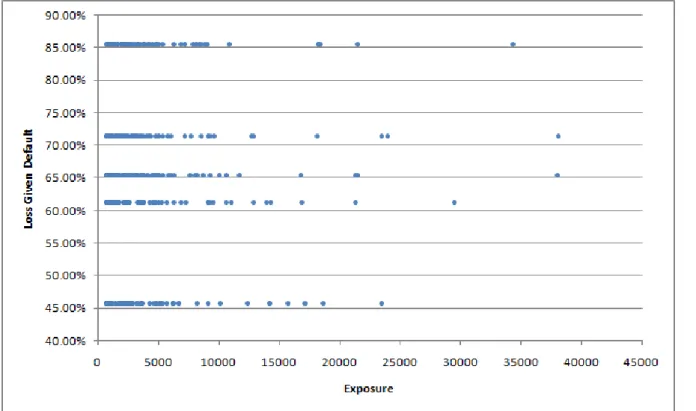
In this thesis, I used a hypothetical portfolio of 500 loans. Each loans are identified by three characteristics; exposure, rating grade and collateral type. I used 16 different rating classes and 5 collateral types. Figure 5 and Figure 6 shows the probability of default vs. exposure size and loss given default vs. exposure size scatters of the portfolio.

33

Figure 5 Probability of default and exposures of loans in the portfolio

Figure 6 Loss given default and exposure of loans in the portfolio

Total exposure of the portfolio is 1.800.000 YTL. Average exposure size of the loans is 3.600 YTL while the median is 2.100 YTL. Hence, exposure distribution of the portfolio is right skewed. The number of the loans below average exposure size exceeds number of the

34

loans that are larger than the average exposure size. Minimum exposure is 700 YTL and maximum exposure is 38.100 YTL.

Distribution of exposure size with respect to both loss given default and probability of default are quite homogenous across different classes. Average exposure among rating classes is 112.500 YTL, while smallest exposure is in A2 rating (90.400 YTL) and largest exposure is in Aa3 rating (134.000 YTL). 4 rating class with lowest PD has slightly larger exposure, than the others. Distribution of collateral types in portfolio is a bit more homogenous than rating classes. Average of exposure size within different collateral types is 360.000 YTL, where the minimum and maximum exposure sizes are 348.000 YTL and 367.400 respectively.

Figure 7 Rating and collateral distribution of the portfolio

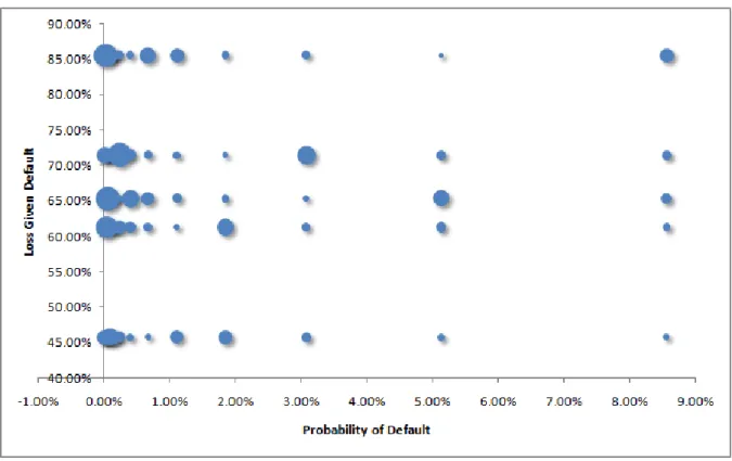
Before simulating the credit risk of the portfolio, let us basically explore the risk profile of the portfolio. In this portfolio, mainly there two sources of uncertainty; probability of default which represents the uncertainty of default event and loss given default that determines the amount of loss when default occurs. Figure 8 shows exposure concentration of the portfolio. In this chart, the larger bubble means the larger exposure in given PD/LGD pair. As we go right and up in the chart the riskiness of exposure increases.

35

Therefore the most risky loans in the portfolio are junior subordinated loans with B3 rating class.

Figure 8 Exposure concentration at each PD/LGD pair

4.2

Models and Assumptions

In the simulation framework of this thesis, there are two model choices; one is for default event and the other is for loss given default. The default models are CreditMetrics and CreditRisk+ as I mentioned in Section 3. LGD models that I consider are; static LGD, stochastic LGD and correlated stochastic LGD model. Under static LGD assumption, I used the average loss given default levels whenever default occurs. Therefore, in this case I add no loss given default uncertainty to the model.

Under stochastic LGD model, the loss given default ratio is a random coming from beta distribution. For each collateral type, a unique distribution is fitted by using average and standard deviation of LGD (for details see Appendix on Beta Distribution).

36

Finally, under correlated stochastic LGD model, loss given default is again a beta distributed random but it is linked with default event as it described in Section 3.3.

The level of default correlation between obligors is very crucial parameter for credit risk calculation. CreditMetrics and CrediRisk+ has different parameters for default correlation. In this thesis I calibrated both models to Basel II’s default correlation model.

In CreditMetrics model, the correlation structure between obligors depend upon the factor loading, 𝑝_𝑗. I can re-write the random term that represents the obligor’s general financial condition (in Section 3.3.1) in terms of correlation with systematic factor;

𝐴𝑗 = 𝜌𝑋 + 1 − 𝜌𝑥𝑗

In Basel II, the default correlation for corporate, sovereign and bank exposures is assumed to be some value from 12% to 24% (Basel Committee on Banking Supervision, 2004). This interval is determined by examining the previous studies and market practice. To calculate the exact level of correlation, Basel II suggests an interpolation formula;

𝜌 = 0.12𝑤 + 0.24 ∗ 1 − 𝑤

where 𝑤 =1−𝑒 −50∗𝑃𝐷

1−𝑒−50 . By this formula, as probability of default increase, the correlation gets closer to 12%. In the limit, if probability of default is exactly one, than 𝜌 becomes 12%. On the other hand, the rating groups with lower probability of default, gets higher correlation. As probability of default decrease, the level of correlation tends to increase. For example, when default probability is zero, the correlation is 24%.

In this thesis, I used Basel’s formula for calculating factor loading, 𝑝_𝑗by using following relation;

37

𝑝2 _{= 𝜌 ⇒ 𝑝 = 𝜌}

There is no direct analog of factor loading in CreditRisk+. In CreditRisk+ default correlation is determined by two parameters, volatility of default probability and weights of correlated shock, 𝑤₁ and 𝑤₂. Therefore I followed a two-step calibration procedure. First, to be able to have weights those are comparable with CreditMetrics’s factor loadings, I used following formula;

𝑤₁ = 𝑝

𝑝 + 1 − 𝑝2 𝑎𝑛𝑑 𝑤2 = 1 − 𝑤1

where 𝑝 is the factor loading in CreditMetrics and it is calculated as explained above. These weights impose the systematic – idiosyncratic factor ratio of CreditMetrics to CreditRisk+ as it is suggested by Altman et al (2005).

In the second step of calibration, I calibrated the volatility of probability of default as it is described in Koyluoglu and Hickman (1998);

𝜎𝑃𝐷 = 𝑃𝐷 1 − 𝑃𝐷 𝜌

where 𝜌 is default correlation and it is calculated by Basel’s formula.

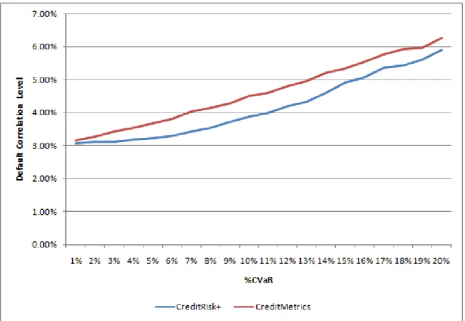
Using this approach, I compared CVaR estimations of two models. To avoid the noise related with the LGD, I used static LGD for this analysis and changed the default correlation level from 1% to 20%. Therefore I run 20 simulations for each model.

38

Figure 9 CVaR% of CreditMetrics and CreditRisk+ with static LGD model at different levels of default correlation

The last parameter that I will mention is the factor loading of the correlated loss given default, 𝑞𝑗. Since the assets of the firm determine both default event and loss, I assumed a level factor loading for LGD which is quite similar to factor loading of the default event, therefore I set 𝑞_𝑗 to 20%. In further results if it is not mentioned, 𝑞_𝑗 is equal to 20%.

4.3

Monte Carlo Simulation

4.3.1 Sketch of Monte Carlo Simulation

In this section I will explain the steps of the Monte Carlo simulation3. The inputs of the simulation software is loan portfolio, default model choice, LGD model choice, LGD correlation level, upper-lower correlation levels for Basel II default correlation formula,