Publisher: Taylor & Francis
Informa Ltd Registered in England and Wales Registered Number: 1072954 Registered office: Mortimer House, 37-41 Mortimer Street, London W1T 3JH, UK
Production Planning & Control
The Management of Operations
Publication details, including instructions for authors and subscription information: http://www.informaworld.com/smpp/title~content=t713737146
An EOQ model for deteriorating items under trade credit
financing in the fuzzy sense
G. C. Mahataa; A. Goswamia
aDepartment of Mathematics, Indian Institute of Technology, Kharagpur, India
Online Publication Date: 01 December 2007
To cite this Article: Mahata, G. C. and Goswami, A. (2007) 'An EOQ model for deteriorating items under trade credit financing in the fuzzy sense', Production Planning & Control, 18:8, 681 - 692
To link to this article: DOI: 10.1080/09537280701619117 URL:http://dx.doi.org/10.1080/09537280701619117
PLEASE SCROLL DOWN FOR ARTICLE
Full terms and conditions of use:http://www.informaworld.com/terms-and-conditions-of-access.pdf
This article maybe used for research, teaching and private study purposes. Any substantial or systematic reproduction, re-distribution, re-selling, loan or sub-licensing, systematic supply or distribution in any form to anyone is expressly forbidden.
Downloaded
B
y:
[
T
he
Indian
Inst
it
ut
e
of
T
echnology]
A
t:
11:
53
27
December
An EOQ model for deteriorating items under
trade credit financing in the fuzzy sense
G. C. MAHATA and A. GOSWAMI*
Department of Mathematics, Indian Institute of Technology, Kharagpur 721302, India
This paper deals with the problem of determining the economic order quantity (EOQ) for deteriorating items in the fuzzy sense where delay in payments for retailer and customer are permissible and generalizes the earlier published results in this direction. The demand rate, holding cost, ordering cost and purchasing cost are taken as fuzzy numbers. We also assume that the supplier would offer the retailer a delay period for payment and the retailer would also offer the trade credit period to the customer. The total variable cost in fuzzy sense is defuzzified using the graded mean integration representation method. Then we have shown that the defuzzified total variable cost is convex, that is, a unique solution exists. For determination of optimal ordering policies, with the help of theorems we have developed the neccessary algorithms. Finally, the theorems and the algorithms are illustrated with the help of numerical examples.
Keywords: EOQ; Fuzzy annual total cost; Trade credit; Graded mean integration representation
1. Introduction
The basic economic order quantity (EOQ) model is based on the implicit assumption that the retailer must pay for the items as soon as he receives them from a supplier. However, in practice, the supplier will allow a certain fixed period (credit period) for settling the amount that the supplier owes to retailer for the items supplied. Before the end of the trade credit period, the retailer can sell the goods and accumulate revenue and earn interest. A higher interest is charged if the payment is not settled by the end of the trade credit period. In the real world, the supplier often makes use of this policy to promote his commodities. In this regard, a number of research papers appeared which deal with the EOQ problem under fixed credit period. Goyal (1985) first studied an EOQ model under the conditions
of permissible delay in payments. Chand and Ward (1987) analysed Goyal’s (1985) problem under assump-tions of the classical EOQ model, obtaining different results. Chung (1998) presented the DCF (discounted cash flow) approach for the analysis of the optimal inventory policy in the presence of trade credit. Later, Shinn et al. (1996) extended Goyal’s (1985) model and considered quantity discount for freight cost. Recently, to accommodate more practical features of the real inventory systems, Aggarwal and Jaggi (1995), Shah (1993), Hwang and Shinn (1997) extended Goyal’s (1985) model to consider the deterministic inventory model with a constant deterioration rate. Shah and Shah (1998) developed a probabilistic inventory model when delay in payment is permissible. They developed an EOQ model for deteriorating items in which time and deterioration of units are treated as continuous variables and demand is a random variable. Later on, Jamal et al. (1997) extended Aggarwal and Jaggi’s (1995) model to allow for shortages and make it more *Corresponding author. Email: [email protected].
ernet.in
Production Planning and Control
ISSN 0953–7287 print/ISSN 1366–5871 onlineß2007 Taylor & Francis http://www.tandf.co.uk/journals
Downloaded
B
y:
[
T
he
Indian
Inst
it
ut
e
of
T
echnology]
A
t:
11:
53
27
December
applicable in the real world. Shawky and Abou-El-Ata (2001) investigated the production lot-size model with both restrictions on the average inventory level and trade credit policy using geometric programming and Lagrange approaches. All the above models assumed that the supplier would offer the retailer a delay period, but the retailer would not offer the trade credit period to his/her customer. Huang (2003) assumed that the retailer should also adopt the trade credit policy to stimulate his/her customer demand to develop the retailer’s replenishment model.
On the other hand, most inventory systems are developed without considering the effects of deteriora-tion. However, in real life situations there are products such as volatile liquids, medicines, materials, etc., in which the rate of deterioration is very large. Therefore, the loss of items due to deterioration should not be neglected. Inventory models for different deteriorating items have been developed by several researchers in past and recent years. Ghare and Schrader (1963) developed an EOQ model for items with an exponentially decaying inventory. An EOQ model for items with variable rate of deterioration has been developed by Covert and Philip (1973) by introducing a two-parameter Weibull distribution for the time to deterioration. Philip (1974) developed a three parameter Weibull distribution for the deterioration time. Many more papers have been published in this direction.
Usually researchers consider different parameters of an inventory model either as constant or dependent on time or probabilistic in nature for the development of the economic order quantity model. But, in the real life situations, these parameters may have little deviations from the exact value which may not follow any probability distribution. In these situations, if these parameters are treated as fuzzy parameters, then it will be more realistic. These types of problems are defuzzified first using a suitable fuzzy technique and then the solution procedure can be obtained in the usual manner. Several authors, namely Chang et al. (1998), Lee and Yao (1998), Lin and Yao (2000), Yao et al. (2000), developed inventory models in fuzzy sense by considering different parameters as fuzzy parameters.
In this paper, we propose a deteriorating inventory model under the condition of permissible delay in payments in the fuzzy sense. Most of the inventory models on this topic assumed that the supplier would offer the retailer a delay period and the retailer could sell the goods and accumulate revenue and earn interest within the trade credit period. They implicitly assumed that the customer would pay for the items as soon as the items are received from the retailer. That is, the retailer would not offer the trade credit period to his/her customer. In most of the business transactions,
this assumption is debatable. In this paper, we assume that the supplier would offer the retailer a delay period and the retailer would also offer the trade credit period to his/her customer. Furthermore, the demand rate and the inventory costs (namely holding cost, purchase cost and ordering cost) may be flexible with some vagueness for their values. In real life situations, all these parameters in an inventory model are uncertain, imprecise and the determination of optimum cycle time becomes a non-stochastic vague decision-making process. Again, for this type of model, statistical estimations proved to be inefficient because of the lack of statistical observations. In this situation, a suitable way to model these imprecise data is to use fuzzy sets. The ill-formed vagueness in the above parameters are introduced making them fuzzy in nature and then the model is formulated in a fuzzy environment. We use the graded mean integration representation method for defuzzifying fuzzy total average cost. In this paper, it is shown that the total variable cost per unit time after defuzzification is convex. Then, with convexity, a simple optimisation procedure is developed. Numerical examples are used to illustrate the results given in this paper. Finally, the results in this paper generalise some already published results in the crisp sense.
2. Assumptions and notations
The mathematical model is developed on the basis of the following assumptions and notations:
(1) The demand rate D is assumed to be constant for the crisp model whereasDeis the fuzzy demand rate for the fuzzy model.
(2) Replenishment rate is infinite and lead time is zero.
(3) Shortage is not allowed.
(4) A constant fraction , assumed to be small, of the on-hand inventory gets deteriorated per unit time.
(5) h, the holding cost per unit; C, the purchasing cost per unit andA, ordering cost per order, are known and constant in the crisp model.eh,Ce, and
e
A are the fuzzy holding cost, fuzzy purchasing cost and fuzzy ordering cost respectively in fuzzy model.
(6) Ic, the interest charged per $ in stocks per year by
the supplier;Ie, the interest earned per $ per year
whereIcIe.
Downloaded
B
y:
[
T
he
Indian
Inst
it
ut
e
of
T
echnology]
A
t:
11:
53
27
December
credit period offered by retailer in years. It is assumed thatMN.
(8) WhenTM, the account is settled at timeT¼M
and retailer starts paying for the interest charges on the items in stock with rateIc. WhenTM,
the account is settled at T¼M and the retailer does not need to pay interest charge.
(9) The retailer can accumulate revenue and earn interest after his/her customer pays for the amount of purchasing cost to the retailer until the end of the trade credit period offered by the supplier. That is, the retailer can accumulate revenue and earn interest during the periodNto
Mwith rateIeunder the condition of trade credit.
3. Crisp mathematical model
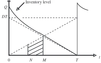
Let q(t) be the inventory level at any time t(0tT). Initially, the stock level is Q. The inventory level decreases due to demand and deterioration until it becomes zero at time t¼T. The differential equation governing the system in the interval (0,T) is
dqðtÞ
dt þqðtÞ ¼ D, 0tT, ð1Þ
with the initial condition
qðTÞ ¼0: ð2Þ
The solution of (1) is
qðtÞ ¼D
eðTtÞ1, 0tT: ð3Þ Using the condition (2), the order quantity can be obtained as
Q¼qð0Þ ¼D
eT1: ð4Þ
Total demand during one cycle isDT.
The number of units deteriorated during one cycle is:
QDT¼D
ðe
T1TÞ: ð5Þ
The total cost due to deterioration of items during the cycle, denoted byDC, is
DC¼CD
eT1T: ð6Þ
The total inventory holding cost per cycle, denoted by
HC, is given by
HC¼h
Z T
0
qðtÞdt¼hD
2
eT1T: ð7Þ
According to assumption (8), three cases may occur in calculation of interest charges for the items kept in stock per year.
Case 1. MT
Total interest payable
¼CIc
ZT M
qðtÞdt
¼CIcD
2
eðTMÞðTMÞ 1: ð8Þ
Case 2. NTM
In this case, total interest payable¼0.
Case 3. TN
Similar as case 2, total interest payable¼0.
According to assumption (9), three cases will occur in interest earned per year.
Case 1. MT, (shown in figure 1)
Total interest earned¼CIe
ZM N
Dtdt
¼CIeDðM 2N2Þ
2 : ð9Þ
Case 2. NTM, (shown in figure 2)
Total interest earned¼CIe
ZT N
DtdtþDTðMTÞ
¼CIeD 2
2MTN2T2: ð10Þ
Case 3. TN, (shown in figure 3)
Total interest earned¼CIeDTðMNÞ: ð11Þ
From the above arguments, the annual total relevant cost for the retailer can be expressed as, TVC(T)¼ ordering cost þ holding cost þ deterioration cost þ
Q
DT
Inventory level
0 N M T t
Downloaded
interest payableinterest earned.
TVCðTÞ ¼
4.1 Graded mean integration representation method
Chen and Hsieh (1999) introduced the graded mean integration representation method based on the integral value of graded meanh-level of the generalised fuzzy number for defuzzifying generalised fuzzy numbers. Here, we first describe the generalised fuzzy number as follows:
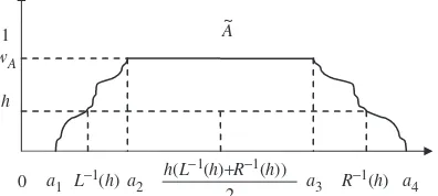
SupposeA~is a generalised fuzzy number as shown in figure 4 and is described as any fuzzy subset of the real line R, whose membership function A~ satisfies the
following conditions:
(1) A~ðxÞ is continuous mapping from R to the
closed interval [0, 1] (2) e
Also this type of generalised fuzzy number may be denoted as Ae¼ ða1,a2,a3,a4;wAÞLR. When wA¼1, it
can be simplified as Ae¼ ða1,a2,a3,a4ÞLR. Second, by
graded mean integration representation methodL1and
R1 are the inverse functions of L and R respectively, and the graded mean h-level value of the generalised fuzzy number A~¼ ða1,a2,a3,a4;wAÞLR is h(L
Let Be be a trapezoidal fuzzy number, and be denoted as Be¼ ðb1,b2,b3,b4Þ. Then we can get the
Figure 2. The total accumulation of interest earned when NTM.
Figure 4. The graded meanh-level value of generalized fuzzy numberA~¼ ða1,a2, a3, a4; wAÞ.
Downloaded
B
y:
[
T
he
Indian
Inst
it
ut
e
of
T
echnology]
A
t:
11:
53
27
December
graded mean integration representation of Be by formula (16) as
PðBeÞ ¼
Z 1
0
hðb1þb4þ ðb2b1b4þb3Þh
2 dh
Z1
0
hdh
¼b1þ2b2þ2b3þb4
6 : ð17Þ
Generalised triangular fuzzy number Xe¼ ða,b,cÞ is a special case of the generalised trapezoidal fuzzy number when b1¼a, b2¼b3¼b and b4¼c. Then by
formula (17), the graded mean integration representa-tion ofXebecomes
PðXeÞ ¼aþ4bþc
6 : ð18Þ
4.2 The fuzzy arithmetical operations under function
principle
Function principle (1985a) is proposed to be as the fuzzy arithmetical operations by triangular fuzzy numbers. We describe some fuzzy arithmetical operations under function principle as follows:
Suppose Ae¼ ða1,a2,a3Þ and Be¼ ðb1,b2,b3Þ are two triangular fuzzy numbers. Then,
(1) The addition ofAeandBeis
e
ABe¼ ða1þb1,a2þb2,a3þb3Þ,
wherea1, a2,a3,b1,b2andb3are any real numbers.
(2) The multiplication ofAeandBeis
e
ABe¼ ða1b1,a2b2,a3b3Þ,
wherea1, a2,a3, b1,b2andb3are all non-zero positive
real numbers.
(3) Be¼ ðb3, b2b1Þ, then the substraction of
e
AandBeis
e
ABe¼ ða1b3,a2b2,a3b1Þ,
wherea1, a2,a3,b1,b2andb3are any real numbers.
(4) Let 2R. Then
ðiÞ Ae¼ ða1,a2,a3Þ, 0
ðiiÞ Ae¼ ða3,a2,a1Þ, 50:
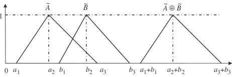
Note: We do not introduce a new addition symbol, as the sum under the extension principle is the same as figure 5. For a mathematically minded reader, we observe that the extension principle is a form of convolution (1985b) while the function principle is akin to a pointwise multiplication as in figure 6.
5. Fuzzy inventory model
In the fuzzy model, we assume that the demand rate, holding cost, purchasing cost and ordering cost are fuzzy numbers and denoted by De, eh, Ce and Ae
respectively. Then the fuzzy annual total relevant cost for the retailer can be expressed as
g
TVCðTÞ ¼
g
TVC1ðTÞ; ifTM,
g
TVC2ðTÞ; ifNTM,
g
TVC3ðTÞ; if 05TN,
8 > > < > > :
ð19Þ
where
g
TVC1ðTÞ ¼X11AeX12ehDeX13CeDe ð20Þ
g
TVC2ðTÞ ¼X21AeX22ehDeX23CeDe ð21Þ
and
g
TVC3ðTÞ ¼X31AeX32heDeX33CeDf, ð22Þ
where
X11 ¼X21 ¼X31¼ 1
T ð23Þ
0 a1 b1 a2 b2 c1 c2 a1a2 b1b2 c1c2
1
A~ B~ A ~⊗ B~
Figure 6. The comparing of fuzzy multiplication operation under function principle and extension principle.
0 a1 a2 b1 b2 a3 b3 a1+b1 a2+b2 a3+b3
1
A~ B~ A ~⊕ B~
Downloaded non-negative triangular fuzzy numbers. Then we get
g the graded mean integration representation ofTVCg1ðTÞ as
Similarly, the graded mean integration representation of
g
Therefore, we have from (19)
PðTVCgðTÞÞ ¼
which is the defuzzified equation corresponding to the equation (19). Then, we have
PðTVCg1ðTÞÞ0¼
where (0) represents differentiation with respect to T.
Downloaded
Before proving Theorem1,we need the following lemmas.
Lemma 1: eTTeT1þ1
The proof of Theorem 1
(1) From equation (35), we have
PðTVCg1ðTÞÞ00
Consider the following equations:
PðTVCg1ðTÞÞ0¼0 ð46Þ
PðTVCg2ðTÞÞ0¼0 ð47Þ
PðTVCg3ðTÞÞ0¼0 ð48Þ
Downloaded
T3 denote the root of equation (48). By the convexity of
PðTVCgiðTÞÞ ði¼1, 2, 3Þ, we see that Decision rule of the optimal cycle time T*:
Theorem 2:
Combining i, ii, iii and equation (33), we have that
PðTVCgðTÞÞ is decreasing on 0, T3 and increasing on Equations (49) imply that
i. PðTVCg1ðTÞÞis increasing on½M,1Þ.
Combining i, ii, iii and equation (33), we have thatPðTVCgðTÞÞ is decreasing on 0, T2 and T2,1.
50. Equations (49) imply that
i. PðTVCg1ðTÞÞ is decreasing on M,T1
Combining i, ii, iii and equation (33), we have that
PðTVCgðTÞÞ is decreasing on 0,T1 and increasing
on T1,1. Consequently, T ¼T1 and
PðTVCgðT ÞÞ ¼PðTVCg1ðT1ÞÞ:
The determination ofT*,T1,T2 andT3 We first describe the following theorem:
Intermediate value theorem: Let f(x) be a continuous function on [a, b] and f(a). f(b)<0, then there exists a
we are in a position to outline the algorithm to findT3.
position to outline the algorithm to findT2.
Downloaded
Then we have the following lemma:
Lemma 3: Suppose that 10 and 2<0, then
1 4M. Consequently, we have com-pleted the proof. By Lemma 3, we are in a position to outline the algorithm to findT1.
Step 1: Let >0. in the fuzzy sense is identical to the cost function (12).
ii. If De¼ ðD,D,DÞ, Ae¼ ðA,A,AÞ, Ce¼ ðC,C,CÞ,
e
Downloaded
Theorem 3: In the crisp case, suppose that the deterioration rate is ignored.
A. If140 and 20,then KðT Þ ¼K3ðT
Theorem 3 has been discussed in Huang (2003).
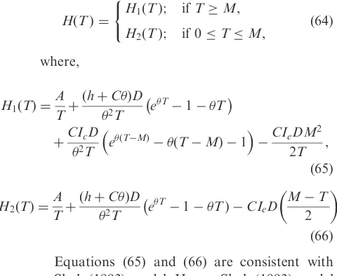
iii. If De¼ ðD,D,DÞ, Ae¼ ðA,A,AÞ, Ce¼ ðC,C,CÞ,
Equations (65) and (66) are consistent with Shah (1993) model. Hence, Shah (1993) model will be a special case of this paper.
iv. If De¼ ðD,D,DÞ, Ae¼ ðA,A,AÞ, Ce¼ ðC,C,CÞ,
e
h¼ ðh,h,hÞ, N¼0 and !0, then the cost function (33) reduces to,
GðTÞ ¼ G1ðTÞ; ifTM,
Equations (68) and (69) are consistent with equations (1) and (4) respectively given in Goyal (1985) model.
8. Numerical examples
To illustrate the results of the proposed method, we solve the following numerical examples.
Let Ae¼$ð94, 100, 108Þ=order, M¼0.1 year,
In this paper, we have developed an EOQ model for deteriorating items in the fuzzy sense where delay in payments for both retailer and customer are permis-sible to reflect realistic situations. We assume that the supplier would offer a trade credit period to the customer. The demand rate and the inventory costs Table 1. The optimal cycle time and total average cost using
Theorem 1.
T* 1 2 PðTVCg3ðT ÞÞ
Downloaded
B
y:
[
T
he
Indian
Inst
it
ut
e
of
T
echnology]
A
t:
11:
53
27
December
(namely holding cost, ordering cost and purchasing cost) are assumed as fuzzy numbers instead of crisp or probabilistic in nature. First, the fuzzy total variable cost is derived. Using the graded mean integration representation method, we have defuzzified the fuzzy total variable cost. Using Theorem 1, it is proved that the defuzzified total variable cost is convex. With the help of Theorem 2 and corresponding lemmas, simple algorithms are provided for obtaining optimum cycle time and total cost. To illustrate different results, numerical examples are provided. Lastly, through some special cases it is shown that earlier published results are special cases of our model.
References
Aggarwal, S.P. and Jaggi, C.K., Ordering policies of deterior-ating items under permissible delay in payments. J. Oper. Res. Soc., 1995,46, 658–662.
Chand, S. and Ward, J., A note on economic order quantity under conditions of permissible delay in payments.J. Oper. Res. Soc., 1987,38, 83–84.
Chang, S.C., Yao, J.S. and Lee, H.M., Economic reorder point for fuzzy backorder quantity.Euro. J. Oper. Res., 1998,109, 183–202.
Chen, S.H. and Hsieh, C.H., Graded mean integration representation of generalized fuzzy number. J. Chinese Fuzzy Syst., 1999,5(2), 1–7.
Chen, S.H., Operations on fuzzy numbers with function principle.Tamkang J. Manage. Sci., 1985a,6(1), 13–26. Chen, S.H., Fuzzy linear combination of fuzzy linear functions
under extension principle and second function principle. Tamsui Oxford J. Manage. Sci., 1985b,1, 11–31.
Covert, R.P. and Philip, G.C., An EOQ model for items with Weibull distribution deterioration. AITE Trans., 1973, 5, 323–326.
Chung, K.J., A theorem on the determination of economic order quantity under conditions of permissible delay in payments.J. Inf. Optim. Sci., 1998,25, 49–52.
Ghare, P.M. and Schrader, G.P., A model for exponentially decaying inventory.J. Indust. Eng., 1963,14, 238–243. Goyal, S.K., Economic order quantity under conditions of
permissible delay in payments.J. Oper. Res. Soc., 1985,36, 335–338.
Hwang, H. and Shinn, S.W., Retailer’s pricing and lot sizing policy for exponentially deteriorating product under the condition of permissible delay in payments. Computer & Oper. Res., 1997,24, 539–547.
Huang, Y.F., Optimal retailer’s ordering policies in the EOQ model under trade credit financing.J. Oper. Res. Soc., 2003, 54, 1011–1015.
Jamal, A.M.M., Sarker, B.R. and Wang, S., An ordering policy for deteriorating items with allowable shortages and permissible delay in payment.J. Oper. Res. Soc., 1997,48, 826–833.
Lee, H.M. and Yao, J.S., Economic production quantity for fuzzy demand quantity and fuzzy production quantity. Euro. J. Oper. Res., 1998,109, 203–211.
Lin, D.C. and Yao, J.S., Fuzzy economic production for production inventory. Fuzzy Sets & Syst., 2000, 111, 465–495.
Philip, G.C., A generalized EOQ model for items with Weibull distribution deterioration.Am. Indust. Eng. Trans., 1974,6, 159–162.
Shah, N.H. and Shah, Y.K., A discrete-in-time probabilistic inventory model for deteriorating items under conditions of permissible delay in payments. Int. J. Syst. Sci., 1998, 29, 121–126.
Shah, N.H., A lot-size model for exponentially decaying inventory when delay in payments is permissible.Cahiers du CERO., 1993,35, 115–123.
Shawky, A.I. and Abou-El-ata, M.O., Constrained production lot-size model with trade-credit policy: a comparison geometric programming approach via Lagrange. Prod. Plan. & Cont., 2001,12, 654–659.
Shinn, S.W., Hwang, H.P. and Sung, S., Joint price and lot size determination under conditions of permissible delay in payments and quantity discounts for freight cost. Euro. J. Oper. Res., 1996,91, 528–542.
Yao, J.S., Chang, S.C. and Su, J.S., Fuzzy inventory without backorder for fuzzy order quantity and fuzzy total demand quantity. Computer & Oper. Res., 2000, 27, 935–962.
Table 2. The optimal cycle time and total average cost using Theorem 1.
T* 1 2 PPðTVCg2ðT ÞÞ
0.01 0.0847568 5121.135 34056.27 661.2437 0.02 0.08248692 6134.910 33045.19 745.7381 0.03 0.08039078 7150.035 32033.45 828.0700 0.04 0.0784472 8166.512 31021.02 908.3977 0.05 0.07663477 9184.342 30007.93 986.8613 0.06 0.07494198 10203.53 28994.16 1063.5850 0.07 0.0733561 11224.07 27979.71 1138.680 0.08 0.0718652 12245.97 26964.59 1212.247 0.09 0.074608 13269.22 25948.79 1284.374 0.10 0.069135 14293.84 24932.32 1355.145
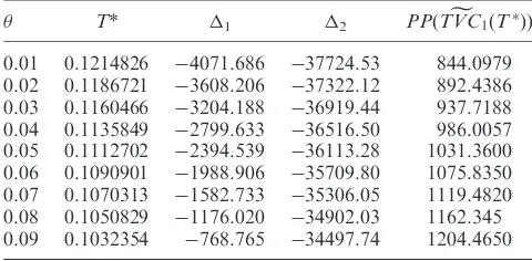
Table 3. The optimal cycle time and total average cost using Theorem 1.
T* 1 2 PPðTVCg1ðT ÞÞ
Downloaded
B
y:
[
T
he
Indian
Inst
it
ut
e
of
T
echnology]
A
t:
11:
53
27
December
G. C. Mahatais a lecturer in the Department of Mathematics at Sitananda College, Nandigram, Purba Medinipur, West Bengal, India. His research interests include inventory management under fuzzy environment and fuzzy optimisation. He has published articles in Computers and Mathematics with Applications, OPSEARCH, etc.