Optimal retailers ordering policies in t

(1)

Abstract—This paper deals with the problem of determining the optimal retailer’s replenishment decisions for deteriorating items under two levels of trade credit policy within the economic order quantity (EOQ) framework to reflect the supply chain management situation. We investigate the retailer's inventory system as a cost minimization problem to determine the retailer's optimal inventory policy under the supply chain management. At first, this paper shows that there exists a unique optimal cycle time to minimize the total variable cost per unit time. Then, a theorem is developed to determine the optimal ordering policies for the retailer. For determination of optimal ordering policies, with the help of theorems, we have developed necessary algorithms. We deduce some previously published results of other researchers as special cases. Finally, numerical examples are given to illustrate the theorems. Then, as well as, we obtain a lot of managerial insights from numerical examples.

Keywords—Deteriorating items, EOQ, Inventory, Trade credit, Permissible delay in payments

I. INTRODUCTION

HE basic EOQ model is based on the implicit assumption that the retailer must pay for the items as soon as he receives them from a supplier. However, in practice, the supplier will allow a certain fixed period (credit period) for settling the amount that the supplier owes to retailer for the items supplied. Before the end of the trade credit period, the retailer can sell the goods and accumulate revenue and earn interest. A higher interest is charged if the payment is not settled by the end of the trade credit period. In a real world, the supplier often makes use of this policy to promote his commodities. In this regard, a number of research papers appeared which deal with the EOQ problem under fixed credit period. Goyal [4] first studied an EOQ model under the conditions of permissible delay in payments. Chand and Ward [2] analyzed Goyal’s [4] problem under assumptions of the classical EOQ model, obtaining different results. Chung [3] presented the DCF (discounted cash flow) approach for the analysis of the optimal inventory policy in the presence of

Gour Chandra Mahata is with the Department of Mathematics, Sitananda College, Nandigram, Purba Medinipur – 721631, West Bengal, INDIA. (corresponding author to provide phone: +91 9474190816; e-mail: [email protected]).

Puspita Mahata is with the department of Commerce, Srikrishna College, Bagula, Nadia - 741502, West Bengal, INDIA.

trade credit. Later, Shinn et al. [12] extended Goyal's [4] model and considered quantity discount for freight cost. Recently, to accommodate more practical features of the real inventory systems, Aggarwal and Jaggi [1], Shah [10], Hwang and Shinn [5] extended Gayal’s [4] model to consider the deterministic inventory model with a constant deterioration rate. Shah and Shah [9] developed a probabilistic inventory model when delay in payment is permissible. They developed an EOQ model for deteriorating items in which time and deterioration of units are treated as continuous variables and demand is a random variable. Later on, Jamal et al. [7] extended Aggarwal and Jaggi’s [1] model to allow for shortages and make it more applicable in real world. Shawky and Abou-El-Ata [11] investigated the production lot-size model with both restrictions on the average inventory level and

trade credit policy using geometric programming and Lagrange approaches. Mahata and Goswami [8] presented a fuzzy EPQ model for deteriorating items when delay in payment is permissible.

All the above models assumed that the supplier would offer the retailer a delay period but the retailer would not offer the trade credit period to his/her customer. In most business transactions, this assumption is unrealistic. Therefore, Huang [6] modified this assumption to assume that the retailer will adopt the trade credit policy to stimulate his/her customer demand to develop the retailer’s replenishment model. Furthermore, it is assumed that the retailer's trade credit period offered by supplier M is not shorter than the customer’s trade credit period offered by retailer N (M ≥N), since the retailer cannot earn any interest in this situation M < N.

Huang [6] implicitly assume that the inventory level is depleted by customer’s demand alone. This assumption is quite valid for non perishable or non deteriorating inventory items. However, there are numerous types of inventory whose utility does not remain constant over time. For example, volatile, liquids, medicines, materials, etc., in which the rate of deterioration is very large. In this case, inventory is depleted not only by customer’s demand but also by the effect of deterioration. Therefore, the loss of items due to deterioration should not be neglected.

In this paper, we want to modify Huang’s [6] model by developing an inventory model for deteriorating items under the condition of permissible delay in payments. We assume that the supplier would offer the retailer a delay period and the

Optimal Retailer’s Ordering Policies in the EOQ

Model for Deteriorating Items under Trade

Credit Financing in Supply Chain

Gour Chandra Mahata and Puspita Mahata

T

International Journal of Mathematical, Physical and Engineering Sciences 3;1 © www.waset.org Winter 2009

(2)

retailer would also offer the trade credit period to his/her customer. We want to relax two assumptions in Huang’s [6] model that unit purchasing cost equals unit selling price, c=s and the inventory level is depleted by customer’s demand alone. Under these conditions, we model the retailer’s inventory system as a cost minimization problem to determine the retailer’s optimal ordering policies.

II. MATHEMATICAL MODEL AND ANALYSIS The mathematical model of the inventory system considered in this paper is basically an extension of the work of Huang [6] and is developed on the basis of the following assumptions and notation:

A. Notation D demand rate per year

θ constant rate of deterioration

A ordering cost per order

c unit purchasing cost per item

s unit selling price per item

Ie interest earned per $ per year

Ic interest charged per $ in stocks per year by the supplier

M the retailer’s trade credit period offered by supplier in years

N the customer’s trade credit period offered by retailer in years

T the cycle time in years (decision variable)

Q procurement quantity (decision variable)

I(t) inventory level at time t (0 ≤ t ≤ T )

C(T) annual total relevant cost, which is a function of T T* the optimal cycle time of C(T)

B. Assumptions

(i) Demand rate, D, is known and assumed to be constant during the cycle time.

(ii) Replenishment rate is infinite and replenishment is instantaneous.

(iii) The lead-time zero. (iv) Shortages are not allowed.

(v) A constant fraction θ, assumed to be small, of the on-hand inventory gets deteriorated per unit time during the cycle time.

(vi) There is no repair or replenishment of deteriorated units in the given cycle.

(vii) s ≥ c, Ic≥ Ie, M ≥ N

(viii) When T ≥ M, the account is settled at time T = M and retailer starts paying for the interest charges on the items in stock with rate Ic. When T ≤ M, the account is settled at T = M and the retailer does not need to pay interest charge.

(ix) The retailer can accumulate revenue and earn interest after his/her customer pays for the amount of purchasing cost to the retailer until the end of the trade credit period offered by the supplier. That is, the retailer can accumulate revenue and earn interest during the period N to M with rate Ie under the condition of trade credit.

C. Mathematical Formulation

The depletion of inventory occurs due to combined effect of the demand and deterioration in the time interval [0; T]. The differential equation governing instantaneous state of I(t) at some instant of time t is given by

T t D

t I dt

t dI

≤ ≤ −

=

+ () , 0

) (

θ , (1)

With the boundary conditions I(0) = Q and I(T) = 0. The solution of (1) is given by

(

1

)

, 0 .

)

(t D e ( ) t T

I = θT−t − ≤ ≤

θ (2)

And the order quantity is

(

1

)

.

) 0

( = −

= T

e D I

Q θ

θ (3) The annual total relevant cost consists of the following elements:

1. Annual ordering cost .

T A =

2. Annual procurement cost = =

(

T −1

)

.

e T cD T

cQ _θ

θ

3. Annual inventory holding cost (excluding interest

charges) () ₂

(

1

)

.

0

T e

T hD dt t I T

h T

T

θ

θ θ − −

= =

_∫

4. According to assumption (viii), three cases may occur in calculation of interest charges for the items kept in stock per year.

Case 1:M≤T.

Annual interest payable

(

1 ( )

)

.

)

( ( )

2 e T M

T D cI dt t I T

cI c T M

T

M

c = − − −

= −

∫

θ

θ θ

Case 2: N≤T ≤M.

In this case, annual interest payable = 0.

Case 3:T ≤N.

Similar as case 2, annual interest payable = 0. 5. According to assumption (ix), three cases will occur

in interest earned.

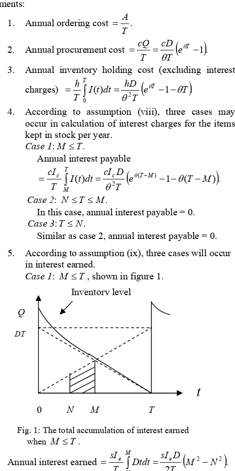
Case 1: M ≤T, shown in figure 1.

Fig. 1: The total accumulation of interest earned when M ≤T.

Annual interest earned

(

)

.

2

2 2

N M T

D sI Dtdt T

sI e

M

N

e = −

=

_∫

Q

DT

Inventory level

0 N M T

t

(3)

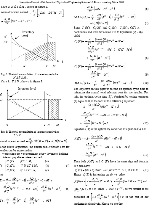
Case 2: N≤T ≤M , shown if figure 2.

Annual interest earned _⎥

⎦

Fig. 2: The total accumulation of interest earned when

M T

N≤ ≤ .

Case 3: T ≤N, shown in figure 3.

Fig. 3: The total accumulation of interest earned when

N

From the above arguments, the annual total relevant cost for the retailer can be expressed as,

C(T) = ordering cost + procurement cost + inventory holding cost + interest payable – interest earned.

⎪⎩

The objective in this paper is to find an optimal cycle time to minimize the annual total relevant cost for the retailer. For this, the optimal cycle time T1*, obtained by setting equation (8) equal to 0, is the root of the following equation: Equation (11) is the optimality condition of equation (5). Let mathematical analysis. Hence we see that

Q

Inventory level

0 T N M

t

(4)

⎪⎪⎩

Based upon the above arguments, we sure that the solution of (11) not only exists but also is unique. Therefore T1* is the

unique non-negative solution of (11). Similarly, the optimal cycle time T2*, obtained by setting equation (9) equal to 0, is the root of the following equation:

+ Equation (15) is the optimality condition of equation (6). Let

+

Therefore, T2* is the unique nonnegative solution of Equation (15) and C2(T)is unimodal as well.

Also, the optimal cycle time T3*, obtained by setting equation (10) equal to 0, is the root of the following equation:

+

Therefore, * 3

T is the unique nonnegative solution of Equation (18) and C3(T) is unimodal as well. Consequently, it is easy

to show the following theorem. Theorem 1:

has the minimum.

III. DECISION RULES OF THE OPTIMAL CYCLE TIME *

T

At present, we will establish an easy procedure to determine the optimal cycle time to simplify the solution procedure. Equations (8) - (10) yield that

Furthermore, we let

)

Generally speaking, Theorem 2 explains that after computing, we can immediately determine which one T1* or

* 2

T or *

3

T is optimal. Theorem 2 gives an analytic method to locate the optimal cycle time of C(T). Using the Intermediate value theorem namely “let g(x) be a continuous function on

[a, b] and g(a)g(b) < 0, then there exists a number c in (a, b)

(5)

(i) Suppose that Δ1>0 and Δ2≥0, then

Consequently, we are in a position to outline the algorithm to find *

3

T denote the root of equation (15). Since

The algorithm to find * 2

Then we have the following lemma:

Lemma 1: Suppose that Δ1≤0 and Δ2 <0, then outline the algorithm to find *

1

IV. SPECIAL CASES 1. Huang’s Model [6]

(6)

)

In this paper, suppose that the selling price per unit and purchase cost per unit are equal and deterioration rate is ignored (θ→0), combining equations (25)-(27), then equations (4 a - c) will be reduced as follows:

⎪⎩

From the viewpoint of the costs, Equations (28a-c) are consistent with Equations (1a-c) in Huang [6] model. Hence, Huang [6] model will be a special case of this paper.

2. Shah’s model [10]

Equations (29 a, b) are consistent with Shah’s [10] model. Hence Shah’s [10] model is a special case of this model. 3. Goyal’ model [4]

Equations (30 a, b) exactly match with equations (1) and (4) in Goyal's model [4], respectively. Hence, Goyal's [4] model is a special case of this model.

V. NUMERICAL EXAMPLES

To illustrate the results of the proposed method, we solve the following numerical examples.

Let A = $150 / order, M = 0.1 year, c = $20 /unit, s = $30 /

Then putting different values for θ, the optimal value of T

and C(T) have been computed. Computed results are displayed in Table 1.

TABLE IIOPTIMAL SOLUTION OF EXAMPLES

Example 1. Case (i): 0 <T ≤N To study the effect of the deterioration rate θon the optimal cycle time T*, on the optimal order quantity Q* and on the optimal annual total cost C(T*) derived by the proposed method, we solve the above three examples with different values of θ. The following observations can be made based on Table 1 which are consistent with our expectation.

(i) The optimal cycle time T* and the optimal order quantity

Q* decrease as the deterioration rate increases.

(ii) The optimal annual total cost C(T*) increases with increase in the decay rate.

(iii) All of T*, Q* and C(T*) being sensitive to changes in the value of the parameter θ, it must be estimated with sufficient care in the real market situations.

VI. CONCLUSION

In reality the value or utility of goods decreases over time for deteriorating items, which in turn suggests smaller cycle length. In this article, we have developed an EOQ model for deteriorating items to determine the optimal ordering policy when the supplier provides the retailer a delay period and the retailer also adopts the trade credit policy to stimulate his / her customer demand to reflect realistic business situations. First, we investigate the retailer's inventory system as a cost minimization problem to determine the retailer's optimal inventory policy under the supply chain management. From the view point of the costs, decision rules to find the optimal cycle time T ¤ contains three cases: (i) T ≤N (ii) N≤T≤M

and (iii) M ≤T. In order to obtain the optimal ordering policy, we propose two theorems and three algorithms. Using

(7)

Theorem 1, it is proved that the annual total variable cost is convex. With the help of Theorem 1 and Theorem 2 and corresponding lemmas, simple algorithms are provided for obtaining the optimum cycle time and the annual total relevant cost. When the deterioration rate is ignored and c = s, Huang’s [6] model can be treated as a special case of this paper. When the customer's trade credit period offered by the retailer equals to zero and c = s, the inventory model discussed in this paper is reduced to Shah’s [10] model. When the customer's trade credit period offered by the retailer equals to zero, c = s and the deterioration rate is ignored, the inventory model discussed in this paper is reduced to Goyal’s [4] model.

Some numerical examples are studied to illustrate the theoretical results. To study the effect of θ on the optimal cycle time T*, on the optimal order quantity Q* and on the optimal annual total cost C(T*), there are some managerial phenomena from Table 1 - Table 3: (i) a higher value of deterioration rate causes lower value of cycle time and order quantity; (ii) a higher value of deterioration rate causes higher value of annual total relevant cost.

The proposed model can assist the retailer in accurately determining the optimal cycle time, the optimal order quantity and the optimal annual total relevant cost. Moreover, the proposed model can be used in inventory control of certain deteriorating items such as food items, photographic film, electronic components, radio active materials, and fashionable commodities, and others.

The proposed model can be extended in several ways. For instance, we may extend the constant deterioration rate to a two-parameter Weibull distribution. In addition, we could consider the replenishment rate as finite, demand as a function of time, selling price, product quality, and others.

APPENDIX

Appendix (A): Proof of theorem 2.

(A) If Δ1 > 0 and Δ2 > 0, then we have f1(M) = f2(M) > 0 and

f1(N) = f2(N) ≥ 0, i.e., ( ) 2/( ) 0 /

1 M =C M >

C and

0 ) ( )

( 3/

/

2 N =C N ≥

C . So T1* <M, T <M

*

2 , T <N *

3 and

N T* <

2 . Equations (14), (17) and (19) imply that (i) C1(T) is increasing on [M, ∞),

(ii) C2(T) is increasing on [N, M], (iii) C3(T) is decreasing on (0, ] * 3

T and increasing on [T3*,N].

Combining (i) - (iii) and equations (4 a - c), we see that C(T)

is decreasing on (0,T3*] and increasing on [ , )

* 3 ∞

T .

Consequently, * 3 *

T

T = and ( ) ( *)

3 *

T C T

C = .

(B) If Δ1 > 0 and Δ2 < 0, then we have f1(M) = f2(M) > 0 and

f1(N) = f2(N) < 0, i.e., ( ) 2/( ) 0 /

1 M =C M >

C and

0 ) ( )

( 3/

/

2 N =C N <

C . So T1* <M, T <M

*

2 , T >N *

3 and

N T* >

2 . Equations (14), (17) and (19) imply that (i) C1(T) is increasing on [M, ∞),

(ii) C2(T) is decreasing on [ , ] * 2

T

N and increasing on

] , [ *

2 M

T ,

(iii) C3(T) is decreasing on (0, N].

* 2 ∞

T .

Consequently, * 2 *

T

T = and ( ) ( *)

2 *

T C T

C = .

(C) If Δ1 ≤ 0 and Δ2< 0, then we have f1(M) = f2(M) ≤ 0 and f1(N) = f2(N) < 0, i.e., ( ) ( ) 0

/ 2 /

1 M =C M ≤

C and

0 ) ( )

( 3/

/

2 N =C N <

C . So T1* >M , T >M

*

2 , T >N *

3 and

N

T2* > . Equations (14), (17) and (19) imply that (i) C1(T) is decreasing on [ , ]

* 1

T

M and increasing on [T1*,∞),

(ii) C2(T) is decreasing on [N, M], (iii) C3(T) is decreasing on (0, N].

* 1 ∞

T .

Consequently, * 1 *

T

T = and ( ) ( *)

1 *

T C T

C = .

REFERENCES

[1] S. P. Aggarwal and C. K. Joggi, “Ordering policies of deteriorating items under permissible delay in Payments”, Journal of Operation Research Society, Vol. 46, 1995, pp. 658 - 662.

[2] S. Chand and J. Ward, “A note on economic order quantity under conditions of permissible delay in payments”, Journal of the Operational Research Society, Vol. 38, 1987, pp. 83 - 84.

[3] K.J. Chung, “A theorem on the determination of economic order quantity under conditions of permissible delay in payments”, J Inf Optim Sci, Vol. 25, 1998, pp. 49 - 52.

[4] S.K. Goyal, “Economic order quantity under conditions of permissible delay in payments”, Journalof Operation Research Society, Vol. 36, 1985, pp. 335 - 338.

[5] H. Hwang and S.W. Shinn, “Retailer's pricing and lot sizing policy for exponentially deteriorating product under the condition of permissible delay in payments”, Computer and Operations Research, Vol. 24, 1997, pp. 539 - 547.

[6] Y.F. Huang, “Optimal retailer's ordering policies in the EOQ model under trade credit financing”, Journal of the Operational Research Society, Vol. 54, 2003, pp. 1011 - 1015.

[7] A.M.M. Jamal, B.R. Sarker and S. Wang, “An ordering policy for deteriorating items with allowable shortages and permissible delay in payment”, Journal of Operation Research Society, Vol. 48, 1997, pp.826 - 833.

[8] G.C. Mahata and A. Goswami, “Production Lot-Size Model with Fuzzy Production Rate and Fuzzy Demand Rate for Deteriorating Item under Permissible Delay in Payments”, OPSEARCH, Vol. 43, No. 4, 2006, pp. 358 - 375.

[9] N.H. Shah and Y.K. Shah, “A discrete-in-time probabilistic inventory model for deteriorating items under conditions of permissible delay in payments”, International Journal of Systems Science, Vol. 29, 1998, pp. 121 - 126.

[10] N.H. Shah, “A lot-size model for exponentially decaying inventory when delay in payments is permissible”, Cahiers du CERO, Vol. 35, 1993, pp. 115 - 123.

[11] A.I. Shawky and M.O. Abou-el-ata, “Constrained production lot-size model with trade-credit policy: a comparison geometric programming approach via Lagrange”, Production Planning and Control, Vol. 12, 2001, pp. 654-659.

[12] S.W. Shinn, H.P. Hwang and S. Sung, “Joint price and lot size determination under conditions of permissible delay in payments and quantity discounts for freight cost”, European Journal of Operational Research, Vol. 91, 1996, pp. 528 - 542.