Vol. 19, No. 1 (2013), pp. 1–14.
THE MISSILE GUIDANCE ESTIMATION USING
EXTENDED KALMAN FILTER-UNKNOWN
INPUT-WITHOUT DIRECT FEEDTHROUGH
(EKF-UI-WDF) METHOD
Subchan
1and Tahiyatul Asfihani
21,2
Institut Teknologi Sepuluh Nopember Sukolilo, Surabaya,
Abstract. This paper consider the estimation of the optimal missile guidance
which the objective is to minimize the interception time and the energy expen-diture. The proposed Extended Kalman Filter-Unknown Input-Without Direct Feedthrough (EKF-UI-WDF) approach is to estimate the optimal missile guidance and the target acceleration as unknown input to the missile-target interception model. Unknown input is any type of signals without prior information from a given state model or a measurement. The computational for the EKF-UI-WDF method and optimal missile guidance show the closest range to the missile-target is smaller than using the EKF. However the Mean Squared Error (MSE) of estimating the optimal missile guidance using EKF method is smaller than using EKF-UI-WDF method.
Key words and Phrases:EKF-UI-WDF, unknown input, optimal control, missile, target.
2000 Mathematics Subject Classification: 93C41
2
Abstrak.Makalah ini mengkaji estimasi panduan optimal peluru kendali. Fungsi tujuannya adalah meminimumkan waktu tembak dan energi yang digunakan peluru kendali. Metode yang digunakan dalam estimasi panduan optimal peluru kendali dan percepatan target adalah metode Extended Kalman Filter-Unknown Input-Without Direct Feedthrough(EKF-UI-WDF), dengan percepatan target sebagai in-put yang tidak diketahui. Inin-put yang tidak diketahui merupakan semua tipe sinyal yang tidak ada informasi sebelumnya dari state model yang diberikan atau penguku-ran. Hasil simulasi dari penerapan metode EKF-UI-WDF dan panduan optimal peluru kendali menunjukkan bahwa jarak terpendek antara peluru kendali dan tar-get yang diperoleh lebih kecil dibandingkan denganExtended Kalman Filter(EKF). Tetapi nilaiMean Squared Error(MSE) estimasi panduan optimal peluru kendali menggunakan metode EKF lebih kecil daripada dengan metode EKF-UI-WDF.
Kata kunci: EKF-UI-WDF, input tidak diketahui, kendali optimal, peluru kendali, target.
1. Introduction
The objective of optimal control problem is to obtain a controller (input signal) subject to dynamic systems and satisfy some constraints by minimizing or maximizing an objective function [6]. In most practical scenarios, there is a need to construct the estimates of state variables which are not available by a direct measurement, especially when they are used in the applications such as the implementation of state feedback controllers.
Extended Kalman Filter (EKF) can be applied to estimate a nonlinear dy-namic model [10]. EKF method is based on linearizing the nonlinear model and the measurement equations with the first order Taylor series expansion. Generally, nonlinear filtering (e.g. EKF method) assume that all inputs are measurable and are not able to jointly estimate unknown inputs and the states [3]. In some cases to get a better estimation it is necessary to estimate the unknown inputs which can be any type of signals without prior information from a given state model. The method which developed from EKF method approach is called Extended Kalman Filter-Unknown Input-Without Direct Feedthrough (EKF-UI-WDF). This method can simultaneously estimates the states and unknown input for nonlinear stochastic discrete-time systems without direct feedthrough from unknown inputs to outputs. A recursive analytical approach of EKF-UI-WDF is derived with the weighted least squares estimation for an extended state vector including the states and unknown inputs.
control energy expenditure and based on the design concept of decreasing the acce-leration requirement commanded in the final phase of engagement is more effective
than APN guidance law withN= 3 [9]. We estimate the optimal missile guidance
with EKF-UI-WDF method and target acceleration is unknown input. For this discussion, the missile-target interception model is explained
2. Missile-Target Interception Model
The 2D missile-target engagement model can be expressed by the following equations [5]:
˙
λ = VTsin (θT −λ)−VMsin (θM −λ)
R (1)
˙
R = VTcos (θT −λ)−VMcos (θM−λ) (2)
˙
θT = aT VT
(3)
˙
θM = aM VM
(4)
and Table 1 shows the variables and parameters of the 2D missile-target engagement model.
Table 1. Variable and Parameter
Symbols
R the relative distance between the missile and target (range)
λ the line-of-sight angle
VT the tangential velocity of the target
VM the tangential velocity of the missile
θT flight path angle of the target
θM flight path angle of the target and the missile
aT the normal acceleration of the target
aM the normal acceleration of the missile
VM the variations, ˙VM = ˜aM
VT the variations, ˙VT = ˜aT
˜
aM the tangential accelerations of the missile
˜
aT the tangential accelerations of the target
3. EKF-UI-WDF Method
4
input is any type of signals without prior information from a given state model or a measurement.
Table 2. Extended Kalman Filter-Unknown Input-Without
Di-rect Feedthrough Algorithm
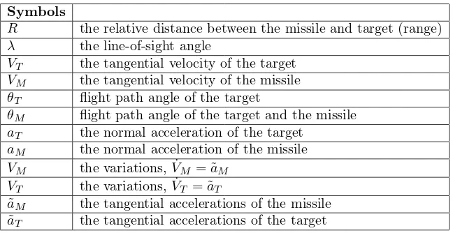
System model and Measurement model Zk =g(
Kalman Gain:
KZ,k=PZ,k|k−1HTk|k−1
Error Covariance:
PZ,k−1|k−1=(In−KZ,k−1Hk−1|k−2)
where
Zk : the states at timekand the value of initialization of the states estimation
is ¯Z0and have covariancePZ0
uk : the known deterministic inputs at timek
u∗k−1 : the unknown inputs at timek
wk−1 : the model noise (uncertainty) have mean ¯wk = 0 and covarianceQk
yk : the measurement vector
vk : the measurement noise have ¯vk= 0 and covarianceRk
Table 2 shows EKF-UI-WDF algorithm which has four parts to estimate
Zk and u∗k−1 at t =k∆t which are denoted as ˆZk|k and ˆu∗k−1|k; respectively. If
unknown inputs are known then EKF-UI-WDF approach becomes EKF method.
4. Optimal Control Solution
Optimal control system of the missile-target interception model based on the design concept of decreasing the acceleration requirement commanded in the final phase of engagement. It is assumed that a perfect knowledge (information) of the
target motion is available to the missile (i.e. VT andaT are known). The objective
function is to minimize the interception time and the control energy expenditure, which can be written as follow
J = tf+ρ
∫ tf
0
aM2dt.
The first term in J is a measure of the interception time, the second term is the
required acceleration command, ρ is the weighting factor reflecting the relative
importance of the commanded acceleration with respect to the interception time.
In general, for short ranges where the time is paramount, the value ofρhas to be
zero, for long ranges where the control energy should be saved so a largerρcan be
chosen.
The solution is derived analytically from the time-varying linear state equa-tions which composed the line-of-sight (LOS) angle and line-of-sight rate. By dif-ferentiating Eq. (1), we obtain the time-varying linear differential equation as
¨
λ = A(t)λ+B(t)aM+C(t)
whereA=−2RR˙ ,B=−cos(λR−θM) andC=aTcos(Rλ−θT).
Defining the statesλ=x1 and ˙λ=x2, then the equations can be defined
˙
x1 = x2 ˙
x2 = A(t)x2+B(t)aM +C(t) (5)
The terminal condition is achieved by
6
and the initial value of states :
x1(0) = x10 x2(0) = x20
Here is the procedure to solve the optimal control problem :
i. Define the Hamiltonian equation : H = 1+ρ aM2+ν1x2+ν2(Ax2+BaM+C)
whereνi is Lagrangian multiplier.
ii. MinimizeH
∂H
∂aM = 0 and obtainedaM =−
Bν2
2ρ .
iii. Using the results aM from (ii) into (i), we obtain the optimal H∗ = 1 +
B2
ν2 2
4ρ +ν1x2+ν2
(
Ax2+−B 2
ν2
2ρ +C
)
.
iv. Solve the differential equations ˙
x(t) =∂ν∂ H∗(x, ν, t)
and co-state equation : ˙ν1 = −∂x∂H1 = 0, ˙ν2 = −
∂H
∂x2 = −ν1−ν2A. The
boundary condition is the initial and final conditions, and it is called the transversality condition [8]. Generally, the boundary conditions for this system are
ν1(tf) = 0 ν2(tf) = ψ
whereψ is an unknown constant. And we obtain
ν1 = 0
ν2 = ψe ∫tf
t Adt
Definingf(t) = e∫ttfAdt, we then have
ν2 = ψf(t) (6)
Thus, Eq. (5) becomes
˙
x2−Ax2=C−
ψB2f(t)
2ρ (7)
Equation (7) is a nonhomegenous differential equation and this solution viewed from the homogen solution and the particular [1], we obtain the following solution
x2(t) =
f(0)
f(t)
(∫ t
0
(
C−
ψ B2f(t)
2ρ
)f(t)
f(0)dt+x20
)
v. Substitute the solutionsx∗,ν∗from (iv) into the expression for the optimal
controlaM from (ii) and substitute the variable from 0 tot. We obtain
aM =
R3λ˙cos (θ
M −λ) +Rcos (θM−λ)∫ttfRaTcos (θT −λ)dt
∫tf
t R2cos2(θM−λ)dt
Eq. (8) shows that the weighting factor ρis not affect explicitly to the controller obtained.
For guidance implementation, the values of the time to go (tgo) in Eq. (8) is
approximate from the following equation
tgo=tf−t∼=−R˙(t)
R(t) (9)
We simplify Eq. (8) with the following assumptions :
i. The tangential velocity of the missile (VM) and the tangential velocity of
the target (VT) are assumed to be constant
ii. The flight path angles of the target and the missile are identical and equal
to the LOS angle (θM =θT =λ).
The relative closing velocityVc is constant (Vc=−R˙), Eq. (8) becomes
aM =
Vc3(tf−t)3λ˙ +Vc(tf−t)∫ttfVc(tf−t)aTdt
∫tf
t Vc 2(t
f−t)2dt
= −3 ˙Rλ˙ +
3
2aT (10)
Eq. (10) is the augmented proportional navigation law with a unitless gain is equal to 3. Therefore, the augmented proportional navigation law is the simplified version of the optimal guidance which we obtain in Eq. (8). After we get the optimal guidance for the missile then we estimate the variables of the control equation in Eq. (8).
5. The EKF-UI-WDF Design
To compute the control in Eq. (8), the estimates ofR,R, λ,˙ λ, θ˙ M, θT andaT
should be obtained by using an appropriate nonlinear filter. For this purpose, the dynamic model in Eqs. (1)-(4) will be transformed into a state space model whose
state and unknown inputs includeR,R, λ,˙ λ, θ˙ M, θT andaT. Taking the derivatives
of ˙R and ˙λ in Eqs (2) and (1), and denoting the states as well as the known and
unknown input asx1 =R, x2 = ˙R, x3 =λ, x4 = ˙λ, x5 =θM, x6 =θT, u=aM
and u∗ =a
T, respectively. We then have the state space model with model noise
used to design of the nonlinear filter as
˙
x1 = x2+w1 (11)
˙
x2 = x42x1+usin (x5−x3)−u∗sin (x6−x3) +w2 (12)
˙
x3 = x4+w3 (13)
˙
x4 = −2x4x2+u
∗cos (x
6−x3)−ucos (x5−x3)
x1
+w4 (14)
˙
x5 = u
VM
8
˙
x6 = u
∗
VT
+w6 (16)
The variations of VM and VT are ˙VM = 0.8 and ˙VT = 0.4.
Substituting (dx/dt)t=k∆t = (xk−xk−1/∆t) [2] into Eqs. (11)-(16) where
xk =x(k∆t) and ∆t is the sampling time interval. We can obtain discrete
non-linear state equation as follows
xk = fk−1(xk−1,uk−1,u∗k−1
)
+wk−1 (17)
where
fk−1= [f1,k−1, f2,k−1, f3,k−1, f4,k−1, f5,k−1, f6,k−1]T
and
f1,k−1 = x2,k−1∆t+x1,k−1
f2,k−1 = (x4,k−12x1,k−1+uk−1sin (x5,k−1−x3,k−1))∆t
−u∗k−1sin (x6,k−1−x3,k−1) ∆t+x2,k−1
f3,k−1 = x4,k−1∆t+x3,k−1
f4,k−1 = −
2x4,k−1x2,k−1+u∗k−1cos (x6,k−1−x3,k−1)
x1,k−1
∆t
−
uk−1cos (x5,k−1−x3,k−1)
x1,k−1
∆t+x4,k−1
f5,k−1 =
uk−1
VM,k−1
∆t+x5,k−1
f6,k−1 = u
∗
k−1
VT ,k−1
∆t+x6,k−1
as well as wk−1 = [w1,k−1, w2,k−1, w3,k−1, w4,k−1, w5,k−1, w6,k−1]T and wk−1 is
the model noise vector (Gaussian white noise,wk−1∼N(0,Qk)).
The measurements for the process model refers to IRS (Inertial Reference
System) of the missile areR,R, λ,˙ λ, θ˙ M andθT, and given by the following
equa-tions
yk =Hxk+vk (18)
wherevk = [v1,k, v2,k, v3,k, v4,k, v5,k, v6,k]T andvk is the measurement noise
vec-tor (Gaussian white noise, vk∼N(0,Rk)) and the matrixH=I6×6.
The estimates of unknown input (u∗
k−1) and state vectors (xk) at t =k∆t
which are denoted as ˆu∗k−1|kand ˆxk|k, respectively. Since the equation (17) are
10
Substituting tf from Eq. (9) to Eq. (8), we obtain the input for discrete
nonlinear filtering as follows
uk−1 =
6. The EKF Design
For comparison, the EKF approach is used in the missile guidance unlike the proposed EKF-UI-WDF approach, because EKF method can not estimate the
joint of states and unknown input. The target acceleration aT estimated with
EKF method has to be treated as a state with assumed dynamics. Thus, the state equations for the design of EKF can be obtained by adding an extra state equation
for theaT to Eqs. (11)-(16) as follow :
dx7
dt =−x7+wT
in whichx7=aT andwT is a Gaussian white noise and replacingu∗ byx7in Eqs.
(11)-(16).
7. Computational Result
This section presents five simulations to show the performances of the EKF-UI-WDF and the EKF for the implementation of optimal missile guidance. The
total time for the simulation run was 2.5sand a time step of ∆t= 0.05swas used.
EKF-UI-WDF Design Parameter. The initial conditions chosen for the model in EKF-UI-WDF design are
ˆ
x0|0= [90,−41,0,0,0, π]T,uˆ∗−1|0= 0
The initial error covariance matrix is
Px,0|0=diag
{
10−1,10−1,10−2,10−2,10−2,10−2}
.
The covariance matrix for the model noisewk−1is chosen to be
Qk−1=diag{
10−4,10−2,10−4,10−2,10−4,10−4}
The covariance matrix for the measurement noisevk is chosen to be
Rk =diag{10−8,10−4,10−8,10−4,10−8,10−8}.
0 0.5 1 1.5 2 2.5
0 50 100
R (m)
0 0.5 1 1.5 2 2.5
−50 −40 −30 −20
Rdot (m/s)
0 0.5 1 1.5 2 2.5
−2 −1 0 1
λ
(rad)
0 0.5 1 1.5 2 2.5
−5 0 5
lambdadot (rad/s)
0 0.5 1 1.5 2 2.5
−2 −1 0 1
θM
(rad)
0 0.5 1 1.5 2 2.5
3.1 3.15 3.2
θ T
(rad)
0 0.5 1 1.5 2 2.5
−10 −5 0 5
time (sec)
u
* (m/s 2 )
0 0.5 1 1.5 2 2.5
−100 −50 0 50
time (sec)
u (m/s
2)
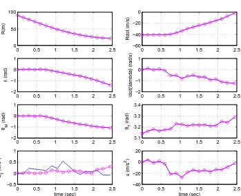
Figure 1. The estimated states and unknown input for the
mis-sile guidance with EKF-UI-WDF (blue curves for real and purple curves for estimation)
Table 3. The MSE (Mean Squared Error) for The Missile Gui-dance Estimation with EKF-UI-WDF Method
Simulation R R˙ λ λ˙
1 9,54.10−9 7,83.10−5 7,17.10−9 8,79.10−5
2 9,38.10−9 6,3.10−5 1,08.10−−8 7,82.10−5
3 1,17.10−8 1,03.10−4 9,14.10−9 7,79.10−5
4 7,86.10−9 8,87.10−5 1,05.10−8 1,09.10−4
5 1,02.10−8 1,4.10−4 1,39.10−8 6,47.10−5
12
Table 4. The MSE (Mean Squared Error) for The Missile Gui-dance Estimation with EKF-UI-WDF Method
Simulation θM θT u∗
1 1,04.10−8 8,42.10−9 8,2161
2 8,98.10−9 1,08.10−8 7,7323
3 9,77.10−9 1,22.10−8 15,8603
4 1,23.10−8 1,04.10−8 12,7958
5 8,34.10−9 1,21.10−8 7,8962
Average 1.10−8 1,08.10−8 10,5
Table 5. The Closest Range Missile-Target with EKF-UI-WDF Method
Simulation The Closest Range Missile-Target (m) Time (s)
1 0 2,45
2 3,338 2,5
3 1,745 2,25
4 0,5487 2,35
5 0,0521 2,5
Average 1,14 2,41
EKF Design Parameter. The initial conditions chosen for EKF design are
ˆ
x0|0= [90,−41,0, 0,0, π,0]T
The initial error covariance matrix is
PZ,0|0=diag{10−1,10−1,10−2,10−2,10−2,10−2,10−2}.
The covariance matrix for the model noisewk−1is chosen to be
Qk−1=diag{
10−4,10−2,10−4,10−2,10−4,10−4,10−2}
. The covariance matrix for the measurement noise is chosen the same for EKF-UI-WDF design.
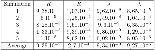
Table 6. The MSE (Mean Squared Error) for The Missile Gui-dance Estimation with EKF Method
Simulation R R˙ λ λ˙
1 9,38.10−9 1,07.10−4 9,62.10−9 8,65.10−5
2 6.10−9 1,25.10−4 1,49.10−8 1,04.10−4
3 8,28.10−9 9,51.10−5 9,3.10−9 6,35.10−5
4 1,33.10−8 9,39.10−4 6,86.10−9 1,29.10−4
5 1.10−8 8,62.10−5 6,02.10−9 8,05.10−5
Average 9,39.10−9 2,7.10−4 9,34.10−9 9,27.10−5
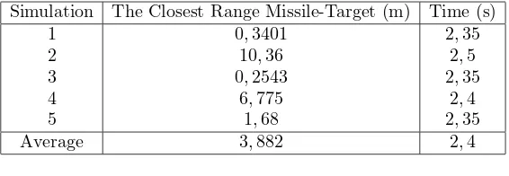
It can be observed from Figures 1-2 that the optimal controller obtained in Eq. (10) with the EKF-UI-WDF method has better interception performance than
the one with the EKF method (the closest missile-target rangesRclosest= 3.338m
0 0.5 1 1.5 2 2.5
Figure 2. The estimated states and target acceleration for the
missile guidance with EKF (blue curves for real and purple curves for estimation)
Table 7. The MSE (Mean Squared Error) for The Missile Gui-dance Estimation with EKF Method
Simulation θM θT aT
14
Table 8. The Closest Range Missile-Target with EKF Method
Simulation The Closest Range Missile-Target (m) Time (s)
1 0,3401 2,35
2 10,36 2,5
3 0,2543 2,35
4 6,775 2,4
5 1,68 2,35
Average 3,882 2,4
8. Concluding Remarks
The solution of the optimal missile guidance is derived analytically from time-varying linear state equations which composed of the line-of-sight angle and rate. The augmented proportional navigation law is the simplified version of the resulting optimal missile guidance which a unitless gain is 3. The computational results of the EKF-UI-WDF method to estimate the optimal missile guidance shows that the range to the missile-target is smaller than using the EKF. However the MSE (Mean Squared Error) for the optimal missile guidance estimation using EKF method is smaller than using EKF-UI-WDF method.
References
[1] Agarwal, P.R. and O’Regan, D.,Ordinary and Partial Differential Equations, Springer, New York, 2009.
[2] Causon, M.D. and Mingham, G.C.,Introductory Finite Difference Methods for PDES, Ventus Publishing, 2010.
[3] Jazwinski, A.H., Stochastic Processes and Filtering Theory, Academic Press, New York, 1970.
[4] Lewis, L.F.,Optimal Estimation with An Introduction to Stochastic Control Theory, Jhon Wiley and Sons, Inc., USA, 1986.
[5] Madyastha, V.K., Adaptive Estimation for Control of Uncertain Nonlinear Systems with Applications to Target Tracking, Ph.D Thesis, School of Aerospace Engineering, Georgia Institute of Technology, USA, 2005.
[6] Naidu, S.D.,Optimal Control System, CRC Press, USA, 2002.
[7] Pan, S., Su, H., Chu, J. and Wang, H., Applying a Novel Extended Kalman Filter to Missile-Target Interception with APN Guidance Law : A Benchmark Case Study,Control Engineer-ing Practice, 159-167, 2010.
[8] Subchan, S. and Zbikowski, R.,Computational Optimal Control Tools and Practise, John Willey and Sons, Ltd., publication, United Kingdom, 2009.
[9] Tsao, L.P. and Lin, C.S., ”A New Optimal Guidance Law for Air-to-Air Missiles against Evasive Targets”,Trans. Japan Soc. Aero. Space Sci.140(2000), 55-60.