El e c t ro n ic
Jo ur
n a l o
f P
r o
b a b il i t y
Vol. 16 (2011), Paper no. 21, pages 587–617. Journal URL
http://www.math.washington.edu/~ejpecp/
Law of large numbers for a class of
random walks in dynamic random environments
∗
L. Avena
1F. den Hollander
1 2F. Redig
1Abstract
In this paper we consider a class of one-dimensional interacting particle systems in equilibrium, constituting a dynamic random environment, together with a nearest-neighbor random walk that on occupied/vacant sites has a local drift to the right/left. We adapt a regeneration-time argument originally developed by Comets and Zeitouni[8]for static random environments to prove that, under a space-time mixing property for the dynamic random environment called cone-mixing, the random walk has an a.s. constant global speed. In addition, we show that if the dynamic random environment is exponentially mixing in space-time and the local drifts are small, then the global speed can be written as a power series in the size of the local drifts. From the first term in this series the sign of the global speed can be read off.
The results can be easily extended to higher dimensions .
Key words: Random walk, dynamic random environment, cone-mixing, exponentially mixing, law of large numbers, perturbation expansion.
AMS 2000 Subject Classification:Primary 60H25, 82C44; Secondary: 60F10, 35B40. Submitted to EJP on March 22, 2010, final version accepted February 10, 2011. 1Mathematical Institute, Leiden University, P.O. Box 9512, 2300 RA Leiden, The Netherlands 2EURANDOM, P.O. Box 513, 5600 MB Eindhoven, The Netherlands
0This paper was written while all three authors were working at the Mathematical Institute
of Leiden University
1
Introduction and main results
In Section 1 we give a brief introduction to the subject, we define the random walk in dynamic random environment, introduce a space-time mixing property for the random environment called cone-mixing, and state our law of large numbers for the random walk subject to cone-mixing. In Section 2 we give the proof of the law of large numbers with the help of a space-time regeneration-time argument. In Section 3 we assume a stronger space-regeneration-time mixing property, namely, exponential mixing, and derive a series expansion for the global speed of the random walk in powers of the size of the local drifts. This series expansion converges for small enough local drifts and its first term allows us to determine the sign of the global speed. (The perturbation argument underlying the series expansion provides an alternative proof of the law of large numbers.) In Appendix A we give examples of random environments that are cone-mixing. In Appendix B we compute the first three terms in the expansion for an independent spin-flip dynamics.
1.1
Background and motivation
In the past forty years, models of Random Walk in Random Environment (RWRE) have been in-tensively studied by the physics and the mathematics community, giving rise to an important and still lively research area that is part of the field of disordered systems. RWRE on Zd is a Random
Walk (RW) evolving according to a random transition kernel, i.e., its transition probabilities depend on a random field or a random processξon Zd called Random Environment (RE). The RE can be eitherstaticordynamic. We refer tostaticRE ifξis chosen at random at time zero and is kept fixed throughout the time evolution of the RW, while we refer todynamic RE when ξchanges in time according to some stochastic dynamics. Forstatic RE, in one dimension the picture is fairly well understood: recurrence criteria, laws of large numbers, invariance principles and refined large de-viation estimates have been obtained in the literature. In higher dimensions many powerful results have been obtained as well, while many questions still remain open. For a review on these results and related questions we refer the reader to[21, 24, 25]. IndynamicRE the state of the art is rather modest even in one dimension, in particular when the RE has dependencies in space and time.
RW in dynamic RE in dimension d can be viewed as RW in static RE in dimension d+1, by con-sidering time as an additional dimension. Consequently, we may expect to be able to adapt tools developed for the static case to deal with the dynamic case as well. Indeed, the proof of our Law of Large Numbers (LLN) in Theorem 1.2 below uses the regeneration technique developed by Comets and Zeitouni for the static case [8] and adapts it to the dynamic case. A number of technicalities become simpler, due to the directedness of time, while a number of other technicalities become harder, due to the lack of ellipticity in the time direction.
Three classes of dynamic random environments have been studied in the literature so far:
(1) Independent in time: globally updated at each unit of time (see e.g. [6, 14, 19]);
(2) Independent in space: locally updated according to independent single-site Markov chains (see e.g.[3, 5]);
(3) Dependent in space and time([1, 2, 7, 9, 10, 12]).
In this paper we focus on models in which the RE are constituted by Interacting Particle Systems (IPS’s). Indeed, IPS’s constitute a well-established research area (see e.g. [15]), and are natural (and physically interesting) examples of RE belonging to class (3). Moreover, results and techniques from IPS’s theory can be used in the present context as in our Theorem 1.3 (see also[2, 9]).
Most known results for dynamic RWRE (like LLN’s, annealed and quenched invariance principles, decay of correlations) have been derived under suitable extra assumptions. Typically, it is assumed either that the random environment has a strong space-time mixing property and/or that the tran-sition probabilities of the random walk are close to constant, i.e., are small perturbation of a homo-geneous RW. Our LLN in Theorem 1.2 is a successful attempt to move away from these restrictions. Cone-mixing is one of the weakest mixing conditions under which we may expect to be able to de-rive a LLN via regeneration times: no rate of mixing is imposed. Still, it is not optimal because it is a
uniformmixing condition (see (1.11)). For instance, the exclusion process, due to the conservation of particles, is not cone-mixing.
Our expansion of the global speed in Theorem 1.3 below, which concerns a perturbation of a homo-geneous RW falls into class (3), but, unlike what was done in previous works, it offers an explicit control on the coefficients and on the domain of convergence of the expansion.
1.2
Model
Let Ω ={0, 1}Z
. Let C(Ω)be the set of continuous functions on Ω taking values in R, P(Ω)the set of probability measures onΩ, and DΩ[0,∞)the path space, i.e., the set of càdlàg functions on
[0,∞)taking values inΩ. In what follows,
ξ= (ξt)t≥0 with ξt={ξt(x): x ∈Z} (1.1)
is an interacting particle system taking values in Ω, i.e., a Feller process on Ω, with ξt(x) = 0
meaning that site x is vacant at timet andξt(x) =1 that it is occupied. The paths ofξtake values
in DΩ[0,∞). The law ofξstarting fromξ0 =η is denoted byPη. The law ofξwhenξ0 is drawn fromµ∈ P(Ω)is denoted byPµ, and is given by
Pµ(·) =
Z
Ω
Pη(·)µ(dη). (1.2)
Through the sequel we will assume that
Pµ is stationary and ergodic under space-time shifts. (1.3)
Thus, in particular,µis a homogeneous extremal equilibrium for ξ. The Markov semigroup associ-ated withξis denoted bySIPS= (SIPS(t))t≥0. This semigroup acts from the left onC(Ω)as
SIPS(t)f
(·) =E(·)[f(ξt)], f ∈C(Ω), (1.4)
and acts from the right onP(Ω)as
νSIPS(t)(·) =Pν(ξt∈ ·), ν∈ P(Ω). (1.5)
Conditional onξ, let
X = (Xt)t≥0 (1.6)
be the random walk with local transition rates
x→x+1 at rate α ξt(x) +β[1−ξt(x)], x→x−1 at rate β ξt(x) +α[1−ξt(x)],
(1.7)
where w.l.o.g.
0< β < α <∞. (1.8)
Thus, on occupied sites the random walk has a local drift to the right while on vacant sites it has a local drift to the left, of the same size. Note that the sum of the jump rates equalsα+β and is thus independent ofξ. Let P0ξ denote the law ofX starting from X0 =0 conditional onξ, which is the
quenchedlaw ofX. Theannealedlaw ofX is
Pµ,0(·) =
Z
DΩ[0,∞)
P0ξ(·)Pµ(dξ). (1.9)
1.3
Cone-mixing and law of large numbers
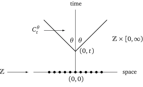
In what follows we will need a mixing propertyfor the law Pµ ofξ. Let (·,·) andk · k denote the inner product, respectively, the Euclidean norm onR2. Putℓ= (0, 1). Forθ ∈(0,1
2π)andt≥0, let
Ctθ =u∈Z×[0,∞): (u−tℓ,ℓ)≥ ku−tℓkcosθ (1.10)
be the cone whose tip is at tℓ= (0,t)and whose wedge opens up in the directionℓwith an angle
θ on either side (see Figure 1). Note that ifθ = 1
2π (θ = 1
4π), then the cone is the half-plane (quarter-plane) abovetℓ.
(0, 0) (0,t)
✲
✲
s s s s s s
s s s s s
θ θ Z×[0,∞)
Z
Ctθ
time
[image:4.612.192.424.474.616.2]space
Figure 1:The coneCtθ.
Definition 1.1. A probability measure Pµ on DΩ[0,∞)satisfying(1.3)is said to be cone-mixing if, for
allθ∈(0,12π),
lim
t→∞ sup
A∈F0,B∈Ftθ
µ(A)>0
Pµ(B|A)−Pµ(B)
where
F0=σξ0(x): x ∈Z ,
Ftθ =σξs(x): (x,s)∈Ctθ .
(1.12)
In Appendix A we give examples of interacting particle systems that are cone-mixing.
We are now ready to formulate our law of large numbers (LLN).
Theorem 1.2. Assume(1.3). If Pµ is cone-mixing, then there exists a v∈Rsuch that
lim
t→∞Xt/t=v Pµ,0−a.s. (1.13)
The proof of Theorem 1.2 is given in Section 2, and is based on aregeneration-time argument origi-nally developed by Comets and Zeitouni[8]for static random environments (based on earlier work by Sznitman and Zerner[22]).
We have no criterion for when v < 0, v = 0 or v > 0. In view of (1.8), a naive guess would be that these regimes correspond to ρ < 12, ρ = 1
2 andρ > 1
2, respectively, with ρ= P
µ(ξ
0(0) =1) the density of occupied sites. However,v= (2 ˜ρ−1)(α−β), with ˜ρthe asymptotic fraction of time spent by the walk on occupied sites, and the latter is a non-trivial function of Pµ,αandβ. We do not (!) expect that ˜ρ= 1
2 whenρ = 1
2 in general. Clearly, if P
µ is invariant under swapping the
states 0 and 1, thenv=0.
1.4
Global speed for small local drifts
For smallα−β, X is a perturbation of simple random walk. In that case it is possible to derive an expansion ofvin powers ofα−β, providedPµsatisfies an exponential space-time mixing property referred to as M < ε(Liggett [15], Section I.3). Under this mixing property, µ is even uniquely ergodic.
Suppose thatξhas shift-invariant local transition rates
c(A,η), A⊂Zfinite,η∈Ω, (1.14)
i.e., c(A,η) is the rate in the configuration η to change the states at the sites in A, and c(A,η) =
c(A+x,τxη)for all x∈Zwithτx the shift of space overx. Define
M =X
A∋0
X
x6=0 sup
η∈Ω
|c(A,η)−c(A,ηx)|,
ε= inf
η∈Ω
X
A∋0
|c(A,η) +c(A,η0)|,
(1.15)
where ηx is the configuration obtained from x by changing the state at site x. The interpretation of (1.15) is thatM is a measure for themaximaldependence of the transition rates on the states of single sites, whileεis a measure for theminimalrate at which the states of single sites change. See Liggett[15], Section I.4, for examples.
Theorem 1.3. Assume(1.3)and suppose that M< ε. Ifα−β < 12(ε−M), then
v= X
n∈N
cn(α−β)n∈R with cn=cn(α+β;Pµ), (1.16)
The proof of Theorem 1.3 is given in Section 3, and is based on an analysis of the semigroup associated with the environment process, i.e., the environment as seen relative to the random walk. The generator of this process turns out to be a sum of a large part and a small part, which allows for a perturbation argument. In Appendix A we show that M < εimplies cone-mixing for spin-flip systems, i.e., systems for whichc(A,η) =0 when|A| ≥2.
It follows from Theorem 1.3 that forα−β small enough the global speedvchanges sign atρ=1
2:
v= (2ρ−1)(α−β) +O (α−β)2asα↓βforρfixed. (1.17)
We will see in Section 3.3 that c2 = 0 when µ is a reversible equilibrium, in which case the error term in (1.17) isO((α−β)3).
In Appendix B we consider an independent spin-flip dynamics such that 0 changes to 1 at rateγand 1 changes to 0 at rateδ, where 0< γ,δ <∞. By reversibility,c2=0. We show that
c3= 4
U2 ρ(1−ρ)(2ρ−1)f(U,V), f(U,V) =
2U+V p
V2+2U V
−p2U+2V
V2+U V
+1, (1.18)
with U = α+β, V = γ+ δ and ρ = γ/(γ+δ). Note that f(U,V) < 0 for all U,V and limV→∞f(U,V) =0 for allU. Therefore (1.18) shows that
(1) c3>0 forρ <12,c3=0 forρ= 12,c3<0 forρ > 12,
(2) c3→0 asγ+δ→ ∞for fixedρ6= 1
2 and fixedα+β.
(1.19)
Ifρ= 1
2, then the dynamics is invariant under swapping the states 0 and 1, so thatv=0. Ifρ > 1 2, then v > 0 for α−β >0 small enough, but v is smaller in the random environment than in the average environment, for which v = (2ρ−1)(α−β) (“slow-down phenomenon”). In the limit
γ+δ→ ∞the walk sees the average environment.
1.5
Extensions
Both Theorem 1.2 and 1.3 are easily extended to higher dimensions (with the obvious generalization of cone-mixing), and to random walks whose step rates are local functions of the environment, i.e., in (1.7) replaceξt(x)byR(τxξt), withτx the shift over x andRany cylinder function onΩ. It is
even possible to allow for steps with a finite range. All that is needed is that the total jump rate is independent of the random environment. The reader is invited to take a look at the proofs in Sections 2 and 3 to see why. In particular, in the context of Theorem 1.3, denote by{e1, . . . ,ed}the
canonical basis ofZd. For anyi=1, . . . ,d, letγi=αi−βi be the local drift in directionei on top of
particles for the RWX in (1.6) extended onZd. Denote byγthed−dimensional vector(γ1, . . . ,γd)
and assume that on vacant sitesX has local drifts−γi along each direction ei. Then Theorem 1.3
still holds under the condition that max{|γi| : i = 1, . . . ,d} < (ε−M)/2 , with asymptotic speed v= (2ρe−1)γ∈Rd.
2
Proof of Theorem 1.2
In this section we prove Theorem 1.2 by adapting the proof of the LLN for random walks instatic
random environments developed by Comets and Zeitouni[8]. The proof proceeds in seven steps. In Section 2.1 we look at a discrete-time random walkX onZin adynamicrandom environment and show that it is equivalent to a discrete-time random walkY on the half-plane
H=Z×N0 (2.1)
in astaticrandom environment that isdirectedin the vertical direction. In Section 2.2 we show that
Y in turn is equivalent to a discrete-time random walk Z onHthat sufferstime lapses, i.e., random times intervals during which it does not observe the random environment and does not move in the horizontal direction. Because of the cone-mixing property of the random environment, these time lapses have the effect ofwiping out the memory. In Section 2.3 we introduceregeneration timesat which, roughly speaking, the future of Z becomes independent of its past. Because Z is directed, these regeneration times are stopping times. In Section 2.4 we derive a bound on the moments of the gaps between the regeneration times. In Section 2.5 we recall a basic coupling property for sequences of random variables that are weakly dependent. In Section 2.6, we collect the various ingredients and prove the LLN for Z, which will immediately imply the LLN for X. In Section 2.7, finally, we show how the LLN forX can be extended fromdiscretetime tocontinuoustime.
The main ideas in the proof all come from[8]. In fact, by exploiting the directedness we are able to simplify the argument in[8]considerably.
2.1
Space-time embedding
Conditional onξ, we define adiscrete-timerandom walk onZ
X = (Xn)n∈N0 (2.2)
with transition probabilities
P0ξ Xn+1=x+i|Xn=x=
pξn+1(x) +q[1−ξn+1(x)] if i=1,
qξn+1(x) +p[1−ξn+1(x)] if i=−1,
0 otherwise,
(2.3)
where x ∈Z, p∈(1
2, 1),q=1−p, and P
ξ
0 denotes the law ofX starting from X0=0 conditional onξ. This is the discrete-time version of the random walk defined in (1.6–1.7), withpandqtaking over the role of α/(α+β) and β/(α+β). Note that the walk observes the environment at the moment when it jumps. As in Section 1.2, we writeP0ξto denote thequenchedlaw ofX andPµ,0to denote theannealedlaw ofX.
Our interacting particle systemξis assumed to start from an equilibrium measureµsuch that the path measure Pµ is stationary and ergodic under space-time shifts and is cone-mixing. Given a realization ofξ, we observe the values ofξat integer timesn∈Z, and introduce a random walk on
H
with transition probabilities
P(0,0)ξ Yn+1=x+e|Yn=x
=
pξx2+1(x1) +q[1−ξx2+1(x1)] ife=ℓ
+,
qξx2+1(x1) +p[1−ξx2+1(x1)] ife=ℓ
−,
0 otherwise,
(2.5)
where x = (x1,x2)∈H,ℓ+= (1, 1),ℓ−= (−1, 1), andPξ
(0,0)denotes the law ofY givenY0= (0, 0) conditional onξ. By construction,Y is the random walk onHthat moves inside the cone with tip at(0, 0)and angle 14π, and jumps in the directions eitherl+orl−, such that
Yn= (Xn,n), n∈N0. (2.6)
We refer toP(0,0)ξ as the quenched law ofY and to
Pµ,(0,0)(·) =
Z
DΩ[0,∞)
P(0,0)ξ (·)Pµ(dξ) (2.7)
as the annealed law ofY. If we manage to prove that there exists au= (u1,u2)∈R2 such that
lim
n→∞Yn/n=u Pµ,(0,0)−a.s., (2.8)
then, by (2.6),u2=1, and the LLN for the discrete-time processY holds withv=u1. In Section 2.7 we show how to pass in continuous time to obtain Theorem 1.2.
2.2
Adding time lapses
PutΛ ={0,ℓ+,ℓ−}. Letε = (εi)i∈N be an i.i.d. sequence of random variables taking values inΛ
according to the product lawW =w⊗Nwith marginal
w(ε1=¯e) =
¨
r if ¯e∈ {ℓ+,ℓ−},
p if ¯e=0, (2.9)
withr= 1
2q. For fixedξandε, introduce a second random walk onH
Z= (Zn)n∈N0 (2.10)
with transition probabilities
¯
P(0,0)ξ,ε Zn+1=x+e|Zn=x
=1{εn+1=e}+
1
p1{εn+1=0}
h
P(0,0)ξ Yn+1= x+e|Yn= x
−r i
, (2.11)
The quenched and annealed laws ofZdefined by
¯
P(0,0)ξ (·) =
Z
ΛN
¯
P(0,0)ξ,ε (·)W(dε), P¯µ,(0,0)(·) =
Z
DΩ[0,∞)
¯
P(0,0)ξ (·)Pµ(dξ), (2.12)
coincide with those ofY, i.e.,
¯
P(0,0)ξ (Z∈ ·) =P(0,0)ξ (Y ∈ ·), P¯µ,(0,0)(Z∈ ·) =Pµ,(0,0)(Y ∈ ·). (2.13)
In words, Z becomes Y when the average over ε is taken. The importance of (2.13) is two-fold. First, to prove the LLN forY in (2.8) it suffices to prove the LLN forZ. Second,Zsuffers time lapses during which its transitions are dictated byεrather thanξ. By the cone-mixing property ofξ, these time lapses will allowξto steadily lose memory, which will be a crucial element in the proof of the LLN forZ.
2.3
Regeneration times
FixL∈2Nand define the L-vector
ε(L)= (ℓ+,ℓ−, . . . ,ℓ+,ℓ−), (2.14)
where the pairℓ+,ℓ−is alternated 12Ltimes. Givenn∈N0andε∈ΛN
with(εn+1, . . . ,εn+L) =ε(L),
we see from (2.11) that (becauseℓ++ℓ−= (0, 2) =2ℓ)
¯
P(0,0)ξ,ε Zn+L= x+Lℓ|Zn= x=1, x ∈H, (2.15)
which means that the stretch of walkZn, . . . ,Zn+Ltravels in the vertical directionℓirrespective ofξ.
Defineregeneration times
τ(0L)=0, τ(kL+1) =infn> τ(kL)+L: (εn−L, . . . ,εn−1) =ε(L) , k∈N. (2.16)
Note that these are stopping times w.r.t. the filtrationG = (Gn)n∈Ngiven by
Gn=σ{εi: 1≤i≤n}, n∈N. (2.17)
Also note that, by the product structure ofW =w⊗Ndefined in (2.9), we haveτ(kL)<∞P¯0-a.s. for
allk∈N.
Recall Definition 1.1 and put
Φ(t) = sup
A∈F0,B∈Ftθ Pµ(A)>0
Pµ(B|A)−Pµ(B)
. (2.18)
Cone-mixing is the property that limt→∞Φ(t) =0 (for all cone anglesθ ∈(0,12π), in particular, for
θ= 1
4πneeded here). Let
Hk=σ(τi(L))ki=0,(Zi)τ (L)
k
i=0,(εi)
τ(kL)−1
i=0 ,{ξt: 0≤t ≤τ
(L)
k −L}
, k∈N. (2.19)
Lemma 2.1. For all L∈2Nand k∈N,P¯µ,(0,0)-a.s.,
P¯µ,(0,0)Z[k]∈ · | Hk−P¯µ,(0,0) Z∈ ·
tv≤Φ(L), (2.20)
where
Z[k]=
Zτ(L)
k +n
−Zτ(L)
k
n∈N
0
(2.21)
andk · ktvis the total variation norm.
Proof. We give the proof fork=1. LetA∈σ(HN0)be arbitrary, and abbreviate 1
A=1{Z∈A}. Leth
be anyH1-measurable non-negative random variable. Then, for all x∈Handn∈N, there exists a random variablehx,n, measurable w.r.t. the sigma-field
σ(Zi)ni=0,(εi)ni=0−1,{ξt: 0≤t<n−L}
, (2.22)
such thath=hx,n on the event{Zn=x,τ
(L)
1 =n}. LetEPµ⊗W and CovPµ⊗W denote expectation and covariance w.r.t.Pµ⊗W, and writeθnto denote the shift of time overn. Then
¯
Eµ,(0,0)
h
1A◦θτ(L)
1
= X
x∈H,n∈N
EPµ⊗W
¯
E0ξ,ε
hx,n[1A◦θn]1nZ
n=x,τ
(L)
1 =n
o
= X
x∈H,n∈N
EPµ⊗W fx,n(ξ,ε)gx,n(ξ,ε)
=E¯µ,(0,0)(h)P¯µ,(0,0)(A) +ρA,
(2.23)
where
fx,n(ξ,ε) =E¯(0,0)ξ,ε
hx,n1n Zn=x,τ
(L)
1 =n
o
, gx,n(ξ,ε) =P¯θnξ,θnε
x (A), (2.24)
and
ρA= X
x∈H,n∈N
CovPµ⊗W fx,n(ξ,ε),gx,n(ξ,ε). (2.25)
By (1.11) and (2.18), we have
|ρA| ≤ X
x∈H,n∈N
CovPµ⊗W fx,n(ξ,ε),gx,n(ξ,ε)
≤ X
x∈H,n∈N
Φ(L)EPµ⊗W fx,n(ξ,ε)sup
ξ,ε
gx,n(ξ,ε)
≤Φ(L) X
x∈H,n∈N
EPµ⊗W fx,n(ξ,ε)= Φ(L)E¯µ,(0,0)(h).
(2.26)
Combining (2.23) and (2.26), we get
E¯µ,(0,0)
h
1A◦θτ(L)
1
−E¯µ,(0,0)(h)P¯µ,(0,0)(A)
≤Φ(L)E¯µ,(0,0)(h). (2.27)
Now pickh=1BwithB∈ H1 arbitrary. Then (2.27) yields
P¯µ,(0,0)Z[k]∈A|B−P¯µ,(0,0)(Z∈A)
≤Φ(L)for allA∈σ(HN0),B∈ H
Therefore, since (2.28) is uniform inB, (2.28) holds ¯Pµ,(0,0)-a.s. whenB is replaced byH1. More-over, (2.28) holds ¯Pµ,(0,0)-a.s. (withH1 in place ofB), simultaneously for all measurable cylinder setsA. Since the total variation norm is defined over cylinder sets, we can take the supremum over
Ato get the claim fork=1.
The extension tok∈Nis straightforward.
2.4
Gaps between regeneration times
Recall (2.16) and thatr= 12q. Define
Tk(L)=rLτ(kL)−τ(kL−)1, k∈N. (2.29)
Note that Tk(L), k∈N, are i.i.d. In this section we prove two lemmas that control the moments of these increments.
Lemma 2.2. For everyα >1there exists an M(α)<∞such that
sup
L∈2N
¯
Eµ,(0,0)
[T1(L)]α≤M(α). (2.30)
Proof. Fixα >1. SinceT1(L)is independent ofξ, we have
¯
Eµ,(0,0)
[T1(L)]α=EW
[T1(L)]α≤ sup
L∈2N
EW
[T1(L)]α, (2.31)
where EW is expectation w.r.t.W. Moreover, for alla>0, there exists a constantC =C(α,a)such
that
[aT1(L)]α≤C eaT1(L), (2.32)
and hence
¯
Eµ,(0,0)
[T1(L)]α≤ C
aα Lsup∈2N
EW
eaT1(L)
. (2.33)
Thus, to get the claim it suffices to show that, forasmall enough,
sup
L∈2N
EW
eaT1(L)
<∞. (2.34)
To prove (2.34), let
I=infm∈N: (εmL, . . . ,ε(m+1)L−1) =ε(L) . (2.35)
By (2.9),I is geometrically distributed with parameterrL. Moreover,τ1(L)≤(I+1)L. Therefore
EWeaT1(L)
=EWearLτ(1L)
≤earLLEWearLI L
=earLLX
j∈N
(earLL)j(1−rL)j−1rL= r
Le2arLL
earLL
(1−rL),
(2.36)
with the sum convergent for 0<a<(1/rLL)log[1/(1−rL)]and tending to zero asL→ ∞(because
Lemma 2.3. lim infL→∞E¯µ,(0,0)(T (L) 1 )>0.
Proof. Note that ¯Eµ,(0,0)(T1(L)) < ∞ by Lemma 2.2. Let N = (Nn)n∈N
0 be the Markov chain with
state spaceS={0, 1, . . . ,L}, starting fromN0=0, such thatNn=swhen
s=0∨maxk∈N: (εn−k, . . . ,εn−1) = (ε (L) 1 , . . . ,ε
(L)
k ) . (2.37)
This Markov chain moves up one unit with probability r, drops to 0 with probability p+r when it is even, and drops to 0 or 1 with probabilityp, respectively,r when it is odd. Sinceτ(1L)=min{n∈
N0: Nn= L}, it follows thatτ(1L)is bounded from below by a sum of independent random variables, each bounded from below by 1, whose number is geometrically distributed with parameter rL−1. Hence
¯
Pµ,(0,0)
τ(1L)≥c r−L≥(1−rL−1)⌊c r−L⌋. (2.38)
Since
¯
Eµ,(0,0)(T1(L)) =rLE¯µ,(0,0)(τ(1L))
≥rLE¯µ,(0,0)
τ(1L)1{τ(L)
1 ≥c r
−L}
≥cP¯µ,(0,0)
τ(1L)≥c r−L
, (2.39)
it follows that
lim inf
L→∞
¯
Eµ,(0,0)(τ(L)
1 )≥ce
−c/r. (2.40)
This proves the claim.
2.5
A coupling property for random sequences
In this section we recall a technical lemma that will be needed in Section 2.6. The proof of this lemma is a standard coupling argument (see e.g. Berbee[4], Lemma 2.1).
Lemma 2.4. Let(Ui)i∈Nbe a sequence of random variables whose joint probability law P is such that,
for some marginal probability lawµ,
P Ui ∈ · |σ{Uj: 1≤ j<i}
−µ(·)
tv≤a a.s. ∀i∈
N. (2.41)
Then there exists a sequence of random variables(Uei,∆i,Ubi)i∈Nsatisfying
(a) (Uei,∆i)i∈Nare i.i.d.,
(b) Uei has probability lawµ,
(c) P(∆i =0) =1−a, P(∆i =1) =a, (d) ∆i is independent ofUbi,
such that
2.6
LLN for Y
Similarly as in (2.29), define
Zk(L)=rL
Zτ(L)
k
−Zτ(L)
k−1
, k∈N. (2.43)
In this section we prove the LLN for these increments and this will imply the LLN in (2.8).
Proof. By Lemma 2.1, we have
P¯µ,(0,0) (Tk(L),Zk(L))∈ · | Hk−1−µ(L)(·)
tv≤Φ(L) a.s. ∀k∈
N, (2.44)
where
µ(L)(A×B) =P¯µ,(0,0) T1(L)∈A,Z1(L)∈B ∀A⊂rLN,B⊂rLH. (2.45)
Therefore, by Lemma 2.4, there exists an i.i.d. sequence of random variables
(Tek(L),Zek(L),∆(kL))k∈N (2.46)
on rLN×rLH× {0, 1}, where (Tek(L),Zek(L)) is distributed according to µ(L) and ∆(kL) is Bernoulli distributed with parameterΦ(L), and also a sequence of random variables
(Tbk(L),Zbk(L))k∈N, (2.47)
such that∆(kL)is independent of(Tbk(L),Zbk(L))and
(Tk(L),Zk(L)) = (1−∆(kL)) (eTk(L),eZk(L)) + ∆(kL)(Tbk(L),Zbk(L)). (2.48)
Let
zL=E¯µ,(0,0)(Z(L)
1 ), (2.49)
which is finite by Lemma 2.2 because|Z1(L)| ≤T1(L).
Lemma 2.5. There exists a sequence of numbers(δL)L∈N0, satisfyinglimL→∞δL=0, such that
lim sup n→∞ 1 n n X k=1
Zk(L)−zL
< δL P¯µ,(0,0)−a.s. (2.50)
Proof. With the help of (2.48) we can write
1
n n X
k=1
Zk(L)= 1
n n X
k=1
e Zk(L)−1
n n X
k=1
∆(kL)eZk(L)+1
n n X
k=1
∆(kL)Zbk(L). (2.51)
By independence, the first term in the r.h.s. of (2.51) converges ¯Pµ,(0,0)-a.s. tozLasL→ ∞. Hölder’s
inequality applied to the second term gives, forα,α′>1 withα−1+α′−1=1,
1 n n X k=1
∆(kL)eZk(L) ≤ 1 n n X k=1 ∆(kL)
α′!
1
α′ 1
n n X k=1 eZk(L)
Hence, by Lemma 2.2 and the inequality|Zek(L)| ≤Tek(L)(compare (2.29) and (2.43)), we have lim sup n→∞ 1 n n X k=1
∆(kL)Zek(L)
≤Φ(L)
1
α′ M(α)
1
α P¯µ,(0,0)−a.s. (2.53)
It remains to analyze the third term in the r.h.s. of (2.51). Define the filtration Gbk =
σ(∆(iL),Zbi(L)):i<k . Since|∆k(L)Zbk(L)| ≤ |Zk(L)|, it follows from Lemma 2.2 that
M(α)≥E¯µ,(0,0)
|∆(kL)Zbk(L)|α|Gbk= Φ(L)E¯µ,(0,0)
|Zbk(L)|α|Gbk a.s. (2.54)
Next, putZbk∗(L)=E¯µ,(0,0)(Zb(L)
k |Gbk)and note that
Mn=
n X
k=1
∆(kL)
k
b
Zk(L)−bZk∗(L) (2.55)
is a mean-zero martingale w.r.t. the filtration Gbn. By the Burkholder-Davis-Gundy inequality (Williams[23], (14.18)), it follows that, forβ=α∧2,
¯
Eµ,(0,0)
sup
n∈N
Mn
β
≤C(β)E¯µ,(0,0) X k∈N
[∆(kL)(bZk(L)−Zbk∗(L))]2
k2
β/2
≤C(β)X
k∈N
¯
Eµ,(0,0) |∆
(L)
k (Zb
(L)
k −bZ
∗(L)
k )|
β
kβ
!
≤C′(β),
(2.56)
for some constantsC(β),C′(β)<∞. HenceMn a.s. converges to an integrable random variable as n→ ∞, and by Kronecker’s lemma (Williams[23], (12.7)),
lim n→∞ 1 n n X k=1
∆(kL)bZk(L)−Zbk∗(L)=0 a.s. (2.57)
Moreover, ifΦ(L)>0, then by Jensen’s inequality and (2.54) we have
|bZk∗(L)| ≤hE¯µ,(0,0)bZk(L)α|Gbki
1
α
≤
M(α)
Φ(L)
1
α a.s.
Hence 1 n n X k=1
∆(kL)bZk∗(L) ≤ M( α) Φ(L)
1 α 1 n n X k=1
∆(kL). (2.58)
As n → ∞, the r.h.s. converges ¯Pµ,(0,0)-a.s. to M(α)1αΦ(L)
1
α′. Therefore, choosing δL = 2M(α)1αΦ(L)
1
α′, we get the claim.
Finally, sinceZek(L)≥rL and
1
n n X
k=1
Lemma 2.5 yields
lim sup
n→∞
1
n Pn
k=1Z (L)
k
1
n Pn
k=1T (L)
k
−zL
tL
<C1δL ¯
Pµ,(0,0)−a.s. (2.60)
for some constantC1 <∞and L large enough. By (2.29) and (2.43), the quotient of sums in the l.h.s. equalsZτ(L)
n /τ (L)
n . It therefore follows from a standard interpolation argument that
lim sup
n→∞
Zn n −
zL tL
<C2δL P¯µ,(0,0)−a.s. (2.61)
for some constantC2<∞andLlarge enough. This implies the existence of the limit limL→∞zL/tL,
as well as the fact that limn→∞Zn/n=uP¯µ,(0,0)-a.s., which in view of (2.13) is equivalent to the statement in (2.8) withu= (v, 1).
2.7
From discrete to continuous time
It remains to show that the LLN derived in Sections 2.1–2.6 for the discrete-time random walk defined in (2.2–2.3) can be extended to the continuous-time random walk defined in (1.6–1.7).
Let χ = (χn)n∈N0 denote the jump times of the continuous-time random walk X = (Xt)t≥0 (with
χ0 =0). LetQdenote the law ofχ. The increments of χ are i.i.d. random variables, independent ofξ, whose distribution is exponential with mean 1/(α+β). Define
ξ∗ = (ξ∗n)n∈N0 with ξ∗n = ξχn,
X∗ = (Xn∗)n∈N
0 with X
∗
n = Xχn.
(2.62)
ThenX∗is a discrete-time random walk in a discrete-time random environment of the type consid-ered in Sections 2.1–2.6, withp=α/(α+β)andq=β/(α+β). Lemma 2.6 below shows that the cone-mixing property ofξcarries over toξ∗under the joint lawPµ×Q. Therefore we have (recall (1.9))
lim
n→∞X ∗
n/n=v
∗ exists(P
µ,0×Q)−a.s. (2.63)
Since limn→∞χn/n=1/(α+β)Q-a.s., it follows that
lim
n→∞Xχn/χn= (α+β)v
∗ exists(P
µ,0×Q)−a.s. (2.64)
A standard interpolation argument now yields (1.13) withv= (α+β)v∗.
Lemma 2.6. Ifξis cone-mixing with angleθ >arctan(α+β), thenξ∗is cone-mixing with angle 14π.
Proof. Fixθ >arctan(α+β), and putc=c(θ) =cotθ <1/(α+β). Recall from (1.10) thatCtθ is the cone with angleθ whose tip is at(0,t). For M ∈N, letCθt,M be the cone obtained fromCθt by extending the tip to a rectangle with baseM, i.e.,
Ctθ,M=Ctθ∪ {([−M,M]∩Z)×[t,∞)}. (2.65)
Becauseξis cone-mixing with angleθ, and
ξis cone-mixing with angleθ and baseM, i.e., (1.11) holds withCtθ replaced byCtθ,M. This is true for everyM∈N.
Define, fort≥0 andM∈N,
Ftθ =σξs(x): (x,s)∈Ctθ ,
Ftθ,M=σξs(x): (x,s)∈Ctθ,M ,
(2.67)
and, forn∈N,
Fn∗=σξ∗m(x): (x,m)∈C
1 4π
n ,
Gn=σχm: m≥n ,
(2.68)
whereC
1 4π
n is the discrete-time cone with tip(0,n)and angle 14π.
Fixδ >0. Then there exists an M =M(δ)∈Nsuch thatQ(D[M])≥1−δwithD[M] ={χn/n≥ c ∀n≥M}. Forn∈N, define
Dn=χn/n≥c ∩σnD[M], (2.69)
where σ is the left-shift acting on χ. Since c < 1/(α+β), we have P(χn/n ≥ c) ≥ 1−δ for
n≥N=N(δ), and henceP(Dn)≥(1−δ)2≥1−2δforn≥N=N(δ),. Next, observe that
B∈ Fn∗=⇒B∩Dn∈ Fcnθ,M⊗ Gn (2.70)
(the r.h.s. is the product sigma-algebra). Indeed, on the eventDn we haveχm≥cmform≥n+M,
which implies that, form≥M,
(x,m)∈C
1 4π
n =⇒ |x|+m≥n=⇒c|x|+χn≥cn=⇒(x,χm)∈Ccnθ,M. (2.71)
Now put ¯Pµ=Pµ⊗Qand, forA∈ F0 withPµ(A)>0 andB∈ Fn∗estimate
|P¯µ(B|A)−P¯µ(B)| ≤I+I I+I I I (2.72)
with
I=|P¯µ(B|A)−P¯µ(B∩Dn|A)|,
I I=|P¯µ(B∩Dn|A)−¯Pµ(B∩Dn)|,
I I I=|P¯µ(B∩D
n)−P¯µ(B)|.
(2.73)
SinceDn is independent ofA,B andP(Dn)≥1−2δ, it follows that I≤2δandI I I ≤2δuniformly inAandB. To boundI I, we use (2.70) to estimate
I I≤ sup A∈F0,B′∈Fθ
cn,M⊗Gn Pµ(A)>0
|¯Pµ(B′|A)−P¯µ(B′)|. (2.74)
But the r.h.s. is bounded from above by
sup A∈F0,B′′∈Fcnθ,M
Pµ(A)>0
because, for everyB′′∈ Fcnθ,M andC ∈ Gn,
|¯Pµ(B′′×C |A)−¯Pµ(B′′×C)|=|[Pµ(B′′|A)−Pµ(B′′)]Q(C)| ≤ |Pµ(B′′|A)−Pµ(B′′)|, (2.76)
where we use thatC is independent ofA,B′′.
Finally, becauseξis cone-mixing with angleθ and baseM, (2.75) tends to zero asn→ ∞, and so by combining (2.72–2.75) we get
lim sup
n→∞
sup A∈F0,B∈F ∗n
Pµ(A)>0
|¯Pµ(B|A)−¯Pµ(B)| ≤4δ. (2.77)
Now letδ↓0 to obtain thatξ∗is cone-mixing with angle 14π.
2.8
Remark on the cone-mixing assumption
We could have tried to follow a shorter approach to deriving the strong LLN in Theorem 1.2, avoid-ing the technicalities of Sections 2.5 and 2.6. Indeed, with the help of the cone-mixavoid-ing assumption and the auxiliary random process Z introduced in Section 2.2, it seems possible to deduce that the environment process, i.e., the environment as seen relative to the random walk (see Defini-tion 3.1), admits a mixing equilibrium measure µe. Consequently, a weak law of large numbers,
L2-convergence, as well as almost-sure convergence with respect toµecan be inferred. If we could
subsequently show that the equilibrium measureµis absolutely continuous with respect toµe, then
Theorem 1.2 would follow. A similar approach has been successfully used in several papers for static and dynamic environments under somewhat stronger assumptions than cone-mixing (see e.g.
[18, 10]). In the present generality it is not trivial to show the absolutely continuity of µe with
respect toµ.
3
Series expansion for
M
< ε
Throughout this section we assume that the dynamic random environmentξfalls in the regime for whichM< ε(recall (1.15)). In Section 3.1 we define theenvironment process, i.e., the environment as seen relative to the position of the random walk. In Section 3.2 we prove that this environment process has a unique ergodic equilibrium µe, and we derive a series expansion forµe in powers of
α−β that converges whenα−β < 12(ε−M). In Section 3.3 we use the latter to derive a series expansion for the global speedv of the random walk.
3.1
Definition of the environment process
LetX = (Xt)t≥0be the random walk defined in (1.6–1.7). Forx ∈Z, letτx denote the shift of space
overx.
Definition 3.1. The environment process is the Markov processζ= (ζt)t≥0with state spaceΩgiven by
where
(τXtξt)(x) =ξt(x+Xt), x ∈Z, t≥0. (3.2)
Equivalently, ifξhas generator LIPS, thenζhas generator L given by
(L f)(η) =c+(η)f(τ1η)− f(η)
+c−(η)f(τ−1η)−f(η)
+ (LIPSf)(η), η∈Ω, (3.3)
where f is an arbitrary cylinder function onΩand
c+(η) =α η(0) +β[1−η(0)],
c−(η) =β η(0) +α[1−η(0)]. (3.4)
LetS = (S(t))t≥0 be the semigroup associated with the generator L. Suppose that we manage to prove thatζ is ergodic, i.e., there exists a unique probability measureµe on Ω such that, for any cylinder function f onΩ,
lim
t→∞(S(t)f)(η) =〈f〉µe ∀η∈Ω, (3.5)
where〈·〉µ
e denotes expectation w.r.t.µe. Then, picking f =φ0withφ0(η) =η(0),η∈Ω, we have lim
t→∞(S(t)φ0)(η) =〈φ0〉µe=ρe ∀η∈Ω (3.6)
for someρe ∈[0, 1], which represents the limiting probability that X is on an occupied site given thatξ0=ζ0=η(note that(S(t)φ0)(η) =Eη(ζt(0)) =Eη(ξt(Xt))).
Next, let Nt+ and Nt− be the number of shifts to the right, respectively, left up to time t in the
environment process. ThenXt=Nt+−N
−
t . SinceM j t =N
j t−
Rt
0 c
j(η
s)ds, j∈ {+,−}, are martingales
with stationary and ergodic increments, we have
Xt=Mt+ (α−β)
Z t
0
2ηs(0)−1
ds (3.7)
withMt= Mt+−Mt− a martingle with stationary and ergodic bounded increments. It follows from (3.6–3.7) that
lim
t→∞Xt/t= (2ρe−1)(α−β) µ−a.s. (3.8)
In Section 3.2 we prove the existence ofµe, and show that it can be expanded in powers ofα−β
whenα−β < 12(ε−M). In particular, it follows from this expansion (see e.g. (3.40)) that µe is
absolutely continuous with respect toµ. In Section 3.3 we use this expansion to obtain an expansion ofρe.
3.2
Unique ergodic equilibrium measure for the environment process
In Section 3.2.1 we prove four lemmas controlling the evolution ofζ. In Section 3.2.2 we use these lemmas to show thatζhas a unique ergodic equilibrium measureµethat can be expanded in powers
ofα−β, providedα−β <12(ε−M).
We need some notation. Letk · k∞ be the sup-norm on C(Ω). Let 9·9 be the triple norm on Ω
defined as follows. Forx ∈Zand a cylinder function f onΩ, let
∆f(x) =sup
η∈Ω
be the maximum variation of f at x, whereηx is the configuration obtained fromηby flipping the state at site x, and put
9f9=X
x∈Z
∆f(x). (3.10)
It is easy to check that, for arbitrary cylinder functions f andgonΩ,
9f g9≤ kfk∞9g9+kgk∞9f9. (3.11)
3.2.1 Decomposition of the generator of the environment process
Lemma 3.2. Assume(1.3)and suppose that M< ε. Write the generator of the environment processζ
defined in(3.3)as
L=L0+L∗= (LSRW+LIPS) +L∗, (3.12)
where
(LSRWf)(η) =12(α+β)
h
f(τ1η) +f(τ−1η)−2f(η)
i ,
(L∗f)(η) =1
2(α−β)
h
f(τ1η)−f(τ−1η)
i
2η(0)−1.
(3.13)
Then L0is the generator of a Markov process that still hasµas an equilibrium, and that satisfies
9S0(t)f9≤e−c t9f9 (3.14)
and
kS0(t)f − 〈f〉µk∞≤Ce−c t9f9, (3.15)
where S0= (S0(t))t≥0 is the semigroup associated with the generator L0, c=ε−M , and C <∞is a
positive constant.
Proof. Note thatLSRWand LIPScommute. Therefore, for an arbitrary cylinder function f on Ω, we have
9S0(t)f9=9et LSRW et LIPSf
9≤9et LIPSf9≤e−c t9f9, (3.16)
where the first inequality uses that et LSRW is a contraction semigroup, and the second inequality
follows from the fact that ξ falls in the regime M < ε (see Liggett [15], Theorem I.3.9). The inequality in (3.15) follows by a similar argument. Indeed,
kS0(t)f − 〈f〉µk∞=ket LSRW et LIPSf
− 〈f〉µk∞≤ ket LIPSf − 〈f〉µk∞≤Ce−c t9f9, (3.17)
where the last inequality again uses thatξ falls in the regime M < ε(see Liggett [15], Theorem I.4.1). The fact thatµis an equilibrium measure is trivial, since LSRWonly acts onηby shifting it.
Note that LSRW is the generator of simple random walk on Z jumping at rateα+β. We view L0 as the generator of an unperturbed Markov process and L∗ as a perturbation of L0. The following lemma gives us control of the latter.
Lemma 3.3. For any cylinder function f onΩ,
kL∗fk∞≤(α−β)kfk∞ (3.18)
and
Proof. To prove (3.18), estimate
kL∗fk∞= 12(α−β)k
f(τ1·)− f(τ−1·)
2φ0(·)−1
k∞
≤ 1
2(α−β)kf(τ1·) +f(τ−1·)k∞≤(α−β)kfk∞.
(3.20)
To prove (3.19), recall (3.13) and estimate
9L∗f9= 12(α−β)9f(τ1·)−f(τ−1·)
2φ0(·)−1
9
≤ 12(α−β)n9f(τ1·)(2φ0(·)−1)9+9f(τ−1·)(2φ0(·)−1)9
o
≤(α−β)
kfk∞9(2φ0−1)9+9f9k(2φ0−1)k∞
= (α−β)kfk∞+9f9≤2(α−β)9f9,
(3.21)
where the second inequality uses (3.11) and the third inequality follows from the fact thatkfk∞≤
9f9for any f such that〈f〉µ=0.
We are now ready to expand the semigroupS ofζ. Henceforth abbreviate
c=ε−M. (3.22)
Lemma 3.4. Let S0= (S0(t))t≥0 be the semigroup associated with the generator L0 defined in(3.13). Then, for any t≥0and any cylinder function f onΩ,
S(t)f = X
n∈N
gn(t,f), (3.23)
where
g1(t,f) =S0(t)f and gn+1(t,f) =
Z t
0
S0(t−s)L∗gn(s,f)ds, n∈N. (3.24)
Moreover, for all n∈N,
kgn(t,f)k∞≤9f9
2(α−β)
c
n−1
(3.25)
and
9gn(t,f)9≤ e−c t[2(α−β)t]
n−1
(n−1)! 9f9, (3.26)
where0!=1. In particular, for all t>0andα−β < 12c the series in(3.23)converges uniformly inη.
Proof. SinceL=L0+L∗, Dyson’s formula gives
et L f =et L0f +
Z t
0
e(t−s)L0L
∗es L fds, (3.27)
which, in terms of semigroups, reads
S(t)f =S0(t)f +
Z t
0
The expansion in (3.23–3.24) follows from (3.28) by induction onn.
We next prove (3.26) by induction onn. For n=1 the claim is immediate. Indeed, by Lemma 3.2 we have the exponential bound
9g1(t,f)9=9S0(t)f9≤e−c t9f9. (3.29)
Suppose that the statement in (3.26) is true up ton. Then
9gn+1(t,f)9=9
Z t
0
S0(t−s)L∗gn(s,f)ds9
≤
Z t
0
9S0(t−s)L∗gn(s,f)9ds
≤
Z t
0
e−c(t−s)9L∗gn(s,f)9ds
=
Z t
0
e−c(t−s)9L∗ gn(s,f)− 〈gn(s,f)〉µ
9ds
≤2(α−β)
Z t
0
e−c(t−s)9gn(s,f)9ds,
≤9f9e−c t[2(α−β)]n
Z t
0
sn−1
(n−1)!ds
=9f9e−c t[2(α−β)t]
n
n! ,
(3.30)
where the third inequality uses (3.19), and the fourth inequality relies on the induction hypothesis.
Using (3.26), we can now prove (3.25). Estimate
kgn+1(t,f)k∞=
Z t
0
S0(t−s)L∗gn(s,f)ds
∞
≤
Z t
0
kL∗gn(s,f)k∞ds
=
Z t
0
L∗ gn(s,f)− 〈gn(s,f)〉µ∞ds
≤(α−β)
Z t
0
gn(s,f)− 〈gn(s,f)〉µ
∞ds
≤(α−β)
Z t
0
9gn(s,f)9ds
≤(α−β)9f9
Z t
0
e−cs [2(α−β)s]
n−1
(n−1)! ds
≤9f92(α−β) c
n
,
where the first inequality uses thatS0(t) is a contraction semigroup, while the second and fourth inequality rely on (3.18) and (3.26).
We next show that the functions in (3.23) are uniformly close to their average value.
Lemma 3.5. Let
hn(t,f) =gn(t,f)− 〈gn(t,f)〉µ, t≥0,n∈N. (3.32)
Then
khn(t,f)k∞≤Ce−c t[2(α−β)t]
n−1
(n−1)! 9f9, (3.33)
for some C<∞(0!=1).
Proof. Note that9hn(t,f)9=9gn(t,f)9fort≥0 andn∈N, and estimate
khn+1(t,f)k∞=
Z t
0
S0(t−s)L∗gn(s,f)− 〈L∗gn(s,f)〉µ
ds
∞
≤C
Z t
0
e−c(t−s)9L∗gn(s,f)9ds
=C
Z t
0
e−c(t−s)9L∗hn(s,f)9ds
≤C2(α−β)
Z t
0
e−c(t−s)9hn(s,f)9ds
≤C9f9e−c t[2(α−β)]n
Z t
0
sn−1
(n−1)!ds
=C9f9e−c t [2(α−β)t]
n
n! ,
(3.34)
where the first inequality uses (3.15), while the second and third inequality rely on (3.19) and (3.26).
3.2.2 Expansion of the equilibrium measure of the environment process
We are finally ready to state the main result of this section.
Theorem 3.6. For α−β < 12c, the environment process ζ has a unique invariant measure µe. In particular, for any cylinder function f onΩ,
〈f〉µ
e=tlim→∞〈S(t)f〉µ=
X
n∈N
lim
Proof. By Lemma 3.5, we have
S(t)f −S(t)fµ ∞= X
n∈N
gn(t,f)− 〈X
n∈N
gn(t,f)〉µ
∞ = X
n∈N
hn(t,f)
∞ ≤ X
n∈N
khn(t,f)k∞≤Ce−c t9f9X n∈N
[2(α−β)t]n
n!
=C9f9e−t[c−2(α−β)].
(3.36)
Since α−β < 12c, we see that the r.h.s. of (3.36) tends to zero as t → ∞. Consequently, the l.h.s. tends to zero uniformly inη, and this is sufficient to conclude that the set I of equilibrium measures of the environment process is a singleton, i.e.,I ={µe}. Indeed, suppose that there are
two e