El e c t ro n ic
Jo ur n
a l o
f P
r o b
a b i l i t y
Vol. 13 (2008), Paper no. 4, pages 79–106. Journal URL
http://www.math.washington.edu/~ejpecp/
Radius and profile of random planar maps with faces
of arbitrary degrees
Gr´egory Miermont CNRS & LM Universit´e de Paris-Sud
Bat. 425, 91405 Orsay Cedex, France.
Mathilde Weill
DMA, ´Ecole normale sup´erieure 45 rue d’Ulm, 75005 Paris, France.
Abstract
We prove some asymptotic results for the radius and the profile of large random planar maps with faces of arbitrary degrees. Using a bijection due to Bouttier, Di Francesco & Guitter between rooted planar maps and certain four-type trees with positive labels, we derive our results from a conditional limit theorem for four-type spatial Galton-Watson trees.
Key words: Random planar map, invariance principle, multitype spatial Galton-Watson tree, Brownian snake.
1
Introduction
1.1 Overview
A planar map is a proper embedding, without edge crossings, of a connected graph in the 2-dimensional sphere S2. Loops and multiple edges are allowed. A map comes with more structure than the original graph, which is given by its faces, i.e. the connected components of the complement of the embedding in S2. If mis a planar map, we write Fm for the set of its faces, andVm for the set of its vertices. The degree deg(f) of a facef ∈ Fm equals the number of edges incident to it, where an edge whose removal disconnects the graph must be counted twice (as it appears twice in a cyclic exploration of its incident face). Arooted planar map is a pair (m, ~e) where m is a planar map and~e is a distinguished oriented edge. The origin o of ~e is called the root vertex. For technical reasons, we also consider thevertex map † made of one vertex bounding a face of degree 0, as a rooted planar map.
Two rooted maps are identified if there exists an orientation-preserving homeomorphism of S2 that sends the first map onto the second, in a way that respects the root edges. With this identification, the setMrof rooted maps is countable, so we can enumerate certain distinguished
subfamilies and sample them at random. Random maps are used in physics, in the field of 2-dimensional quantum gravity, as discretized versions of an ill-defined random surface [2]. On a mathematical level, this requires a detailed understanding of geometric properties of maps. One possible approach is to consider maps as metric spaces by endowing the set of their vertices with the usual graph distance: if aand a′ are two vertices of a map m,d(a, a′) is the minimal number of edges on a path fromatoa′.
The laws on maps that we want to consider are Boltzmann laws parameterized by a sequence
q = (qi, i≥ 1) of nonnegative weights such that qi > 0 for at least one i≥ 3. For any planar
mapm, we defineWq(m) by Wq(†) = 1 and
Wq(m) = Y
f∈Fm
qdeg(f).
Our basic assumption is that qis be admissible, that is
Zq= X m∈Mr
#VmWq(m)<∞.
In this case, we let
Zq(r)=
X
m∈Mr
Wq(m)<∞,
and define the Boltzmann probability distributionBrq on the setMr by
Brq({m}) = Wq(m) Zq(r)
.
Our main goal is to obtain asymptotic results for certain geometric functionals ofBrq-distributed maps conditioned to have a large number of vertices. The typical quantities of interest will be the radiusRm of the mapm, defined as the maximal distance betweenoand another vertex of
and the profile ofm, which is the measureλm on {0,1,2, . . .} defined by
λm({k}) = #{a∈ Vm :d(o, a) =k}, k ≥0.
Note that Rm is the supremum of the support of λm. It is also convenient to introduce the rescaled profile. Ifm hasnvertices, this is the probability measure onR+ defined by
λ(n)m (A) =
λm(n1/4A) n
for any Borel subsetAofR+. Theorem 1.2 below provides the limits in distribution forn−1/4Rm andλ(n)m under the measureBrq conditioned on{Vm =n}asn→ ∞, for a wide class of weights
q. The limiting distributions are given in terms of the so-called one-dimensional Brownian snake driven by a normalized excursion. For instance, the limiting distribution of the renormalized radius is a multiple of the range of the Brownian snake. The latter is a continuous limit of models of spatial trees which was introduced by Le Gall, and is also related to the so-called ISE of Aldous.
Such results were obtained earlier by Chassaing & Schaeffer in the pioneering work [4] in the special case of quadrangulations, corresponding to the case q4 = 1 andqi = 0 for i6= 4, and by
Weill [19] in the case of bipartite maps where qi = 0 for odd i. Similar results are proved in
Marckert & Miermont [14] for bipartite maps and in Miermont [17] for the general case, but in quite different settings. Indeed [14] and [17] deal with maps that are both rooted and pointed (see definitions below), and consider distances from the distinguished point rather that from the root vertex.
1.2 Setting
1.2.1 Assumptions on q
Since Boltzmann distributions on bipartite maps have been the object of [17], we will assume from now on that q2κ+1>0 for someκ≥1.
We first need to define some auxiliary material. Arooted pointedplanar map is a triple (m, τ, ~e) where (m, ~e) is a rooted planar map andτ is a distinguished vertex. We let Mr,p be the set of
rooted, pointed planar maps, and allow† among its elements. In what follows, we will focus on the subsetM+r,p of Mr,p defined by :
M+r,p ={(m, τ, ~e)∈ Mr,p :d(τ, ~e+) =d(τ, ~e−) + 1} ∪ {†},
where~e−, ~e+are the origin and target of the oriented edge~e. Note that the quantityZqdefined
above also equals
Zq= X
(m,τ,~e)∈Mr,p
Wq(m),
because the choice of any vertex in a rooted map yields a distinct element ofMr,p. Set also
Zq+= X
(m,τ,~e)∈M+r,p
Wq(m).
Ifq is admissible, then this quantity is finite as well, we define the Boltzmann distribution B+q on the setM+r,p by
B+q({m}) = Wq(m) Zq+
.
The family of weightsqthat we consider is the same as in [17], and we recall it briefly here. For k, k′ ≥ 0 we set N•(k, k′) = 2k+k
. For every weight sequence we define
From Proposition 1 in [17], a sequenceq is admissible if and only if the system
has a spectral radius̺≤1. Furthermore this solution is unique and
z+ = Zq+,
z♦ = Zq♦,
where (Z♦
q)2 =Zq−2Zq++ 1. An admissible weight sequenceqis said to becriticalif the matrix Mq(Zq+, Zq♦) has a spectral radius ̺= 1. An admissible weight sequenceqis said to be regular criticalifq is critical and iff•
q(Zq++ε, Zq♦+ε)<∞ for someε >0.
1.2.2 The Brownian snake and the conditioned Brownian snake
Letx∈R. The Brownian snake with initial pointxis a pair (b,rx), whereb= (b(s),0≤s≤1) is a normalized Brownian excursion and rx = (rx(s),0 ≤ s ≤ 1) is a real-valued process such that, conditionally givenb,rx is Gaussian with mean and covariance given by
• E[rx(s)] =x for everys∈[0,1],
• Cov(rx(s),rx(s′)) = inf
s≤t≤s′b(t) for every 0≤s≤s ′ ≤1.
We know from [7] thatrx admits a continuous modification. From now on we consider only this modification. In the terminology of [7]rx is the terminal point process of the one-dimensional Brownian snake driven by the normalized Brownian excursionb and with initial pointx. Write Pfor the probability measure under which the collection (b,rx)x∈R is defined. As men-tioned in [19], for everyx >0, we have
P
inf
s∈[0,1]r
x(s)≥0
>0.
We may then define for everyx >0 a pair (bx,rx) which is distributed as the pair (b,rx) under the conditioning that infs∈[0,1]rx(s)≥0.
We equipC([0,1],R)2with the normk(f, g)k=kfk
u∨kgku wherekfkustands for the supremum
norm off. The following theorem is a consequence of Theorem 1.1 in Le Gall & Weill [13].
Theorem 1.1. There exists a pair (b0,r0) such that(bx,rx) converges in distribution as x↓0 towards (b0,r0).
The pair (b0,r0) is the so-called conditioned Brownian snake with initial point 0. Theorem 1.2 in [13] provides a useful construction of the conditioned object (b0,r0) from the unconditioned one (b,r0). This construction also appears in Marckert & Mokkadem [15], though its outcome was not interpreted as the object appearing in Theorem 1.1. First recall that there is a.s. a uniques∗ in (0,1) such that
r0(s∗) = inf
s∈[0,1]r 0(s)
constructed explicitly as follows : for every s∈[0,1],
b0(s) = b(s∗) +b({s∗+s})−2 inf
s∧{s∗+s}≤t≤s∨{s∗+s}
b(t),
r0(s) = r0({s∗+s})−r0(s∗).
1.3 Statement of the main result
Recall from section 1.2.2 that (b,r0) denotes the Brownian snake with initial point 0.
Theorem 1.2. Let q be a regular critical weight sequence. There exists a scaling constant Cq such that the following results hold.
(i) The law ofn−1/4Rm underBqr(· |#Vm =n)converges asn→ ∞to the law of the random variable
Cq
sup
0≤s≤1
r0(s)− inf
0≤s≤1r 0(s)
.
(ii) The law of the random probability measure λ(n)m under Brq(· | #Vm = n) converges as n→ ∞ to the law of the random probability measure I defined by
hI, gi=
Z 1
0
g
Cq
r0(t)− inf
0≤s≤1r 0(s)
dt.
(iii) The law of the rescaled distance n−1/4d(o, a) where a is a vertex chosen uniformly at random among all vertices of m, under Brq(· | #Vm =n) converges as n→ ∞to the law of the random variable
Cq sup
0≤s≤1
r0(s).
Theorem 1.2 is analogous to Theorem 2.5 in [19] in the setting of non-bipartite maps. Beware that in Theorem 1.2 maps are conditioned on their number of vertices whereas in [19] they are conditioned on their number of faces. However the results stated in Theorem 2.5 in [19] remain valid by conditioning on the number of vertices (with different scaling constants). On the other hand, our arguments to prove Theorem 1.2 do not lead to the statement of these results by conditioning maps on their number of faces. A notable exception is the case of k-angulations (q=qδk for somek≥3 and appropriate q >0), where an application of Euler’s formula shows
that #Fm = (k/2−1)#Vm + 2, so that the two conditionings are essentially equivalent and result in a change in the scale factor Cq.
Recall that the results of Theorem 2.5 in [19] for the special case of quadrangulations were obtained by Chassaing & Schaeffer [4] (see also Theorem 8.2 in [9]). Last, observe that Theorem 1.2 is obviously related to Theorem 1 in [17]. Note however that [17] deals with rooted pointed maps instead of rooted maps as we do and studies distances from the distinguished point of the map rather than from the root vertex.
2
Preliminaries
2.1 Multitype spatial trees
We start with some formalism for discrete trees. Set
U = [
n≥0
Nn,
where by convention N = {1,2,3, . . .} and N0 = {∅}. An element of U is a sequence u = u1. . . un, and we set |u| = n so that |u| represents the generation of u. In particular |∅| = 0. If u = u1. . . un and v = v1. . . vm belong to U, we write uv = u1. . . unv1. . . vm for the
concatenation of u and v. In particular ∅u = u∅ = u. If v is of the form v = uj for u ∈ U and j∈N, we say thatv is a child of u, or that u is the father ofv, and we writeu= ˇv. More generally if v is of the form v =uw foru, w ∈ U, we say that v is a descendant of u, or that u is an ancestor of v. The set U comes with the natural lexicographical order such that u4v if eitheru is an ancestor ofv, or ifu=waand v=wb witha∈ U∗ andb∈ U∗ satisfying a1< b1, where we have setU∗ =U \ {∅}. We writeu≺v ifu4v andu6=v.
A plane treet is a finite subset of U such that
• ∅∈t,
• u∈t\ {∅} ⇒uˇ∈t,
• for everyu∈t there exists a numbercu(t)≥0 such that uj ∈t⇔1≤j≤cu(t).
Let t be a plane tree and let ξ = #t −1. The search-depth sequence of t is the sequence u0, u1, . . . , u2ξ of vertices of twhich is obtained by induction as follows. Firstu0 =∅, and then
for every i∈ {0,1, . . . ,2ξ−1}, ui+1 is either the first child of ui that has not yet appeared in
the sequenceu0, u1, . . . , ui, or the father ofui if all children ofuialready appear in the sequence
u0, u1, . . . , ui. It is easy to verify that u2ξ =∅and that all vertices of t appear in the sequence
u0, u1, . . . , u2ξ (of course some of them appear more than once). We can now define the contour
functionoft. For everyk∈ {0,1, . . . ,2ξ}, we letC(k) =|uk|denote the generation of the vertex
uk. We extend the definition of C to the line interval [0,2ξ] by interpolating linearly between
successive integers. Clearlyt is uniquely determined by its contour functionC.
Let K ∈N and [K] ={1,2, . . . , K}. A K-type tree is a pair (t,e) where t is a plane tree and
e:t→[K] assigns a type to each vertex. If (t,e) is a K-type tree and if i∈[K] we set
ti={u∈t:e(u) =i}.
We denote byT(K) the set of allK-type trees and we set
Ti(K) =n(t,e)∈T(K):e(∅) =io.
Set
WK=
[
n≥0
with the convention [K]0 ={∅}. An element ofWK is a sequencew= (w1, . . . , wn) and we set
|w|=n. Consider the natural projection p:WK→Z+K wherep(w) = (p1(w), . . . , pK(w)) and
pi(w) = #{j∈ {1, . . . ,|w|}:wj =i}.
Note thatp(∅) = (0, . . . ,0) with this definition. Letu∈ U and let (t,e)∈T(K)such thatu∈t.
We then definewu(t)∈ WK by
wu(t) = (e(u1), . . . ,e(ucu(t))),
and we setzu(t) =p(wu(t)).
AK-type spatial tree is a triple (t,e,ℓ) where (t,e)∈T(K) and ℓ:t→R. Ifv is a vertex oft,
we say thatℓv is thelabelofv. We denote byT(K)the set of allK-type spatial trees and we set
T(K)i =n(t,e,ℓ)∈T(K):e(∅) =io.
If (t,e,ℓ) ∈ T(K) we define the spatial contour function of (t,e,ℓ) as follows. Recall that u0, u1, . . . , u2ξ denotes the search-depth sequence of t. First if k∈ {0, . . . ,2ξ}, we put V(k) =
ℓuk. We then complete the definition ofV by interpolating linearly between successive integers.
2.2 Multitype spatial Galton-Watson trees
Letζ = (ζ(i), i∈[K]) be a family of probability measures on the setWK. We associate with ζ
the familyµ= (µ(i), i∈[K]) of probability measures on the setZK+ in such a way that eachµ(i) is the image measure ofζ(i) under the mapping p. We make the basic assumption that
max
i∈[K]µ (i)
(
z∈ZK+ :
K
X
j=1
zj 6= 1
)!
>0,
and we say thatζ (orµ) is non-degenerate. If for everyi∈[K],w∈ WK andz=p(w) we have
ζ(i)({w}) = µ
(i)({z})
# (p−1(z)),
then we say thatζ is theuniform ordering of µ. For everyi, j ∈[K], let
mij =
X
z∈ZK
+
zjµ(i)({z}),
be the mean number of type-j children of a type-iindividual, and letMµ= (mij)1≤i,j≤K. The
matrixMµ is said to be irreducible if for everyi, j∈[K] there existsn∈N such thatm(n)ij >0
where we have written m(n)ij for the ij-entry of Mnµ. We say thatζ (or µ) is irreducible if Mµ
is. Under this assumption the Perron-Frobenius theorem ensures that Mµ has a real, positive
Assume that ζ is non-degenerate, irreducible and (sub-)critical. We denote byPζ(i) the law of a K-type Galton-Watson tree with offspring distribution ζ and with ancestor of typei, meaning that for every (t,e)∈Ti(K),
Pζ(i)({(t,e)}) =Y
u∈t
ζ(e(u))(w u(t)),
The fact that this formula defines a probability measure onTi(K) is justified in [16].
Let us now recall from [16] how one can couple K-type trees with a spatial displacement in order to turn them into random elements ofT(K). To this end, consider a family ν = (νi,w, i∈
[K],w∈ WK) whereνi,wis a probability measure onR|w|. If (t,e)∈T(K)andx∈R, we denote by Rν,x((t,e),dℓ) the probability measure on Rt which is characterized as follows. For every
i ∈[K] and u ∈ t such that e(u) = i, consider Yu = (Yu1, . . . , Yu|w|) (where we have written
wu(t) = w) a random variable distributed according toνi,w, in such a way that (Yu, u∈t) is
a collection of independent random variables. We setL∅=x and for everyv∈t\ {∅},
Lv =
X
u∈]]∅,v]]
Yu,
where ]]∅, v]] is the set of all ancestors of v distinct from the root ∅. The probability measure Rν,x((t,e),dℓ) is then defined as the law of (Lv, v ∈ t). We finally define for every x ∈ R a
probability measureP(i)ζ,ν,x on the setT(K)i by setting,
P(i)ζ,ν,x(dtdedℓ) =Pζ(i)(dt,de)Rν,x((t,e),dℓ).
2.3 The Bouttier-Di Francesco-Guitter bijection
We start with a definition. We consider the set TM ⊂T1(4) of 4-type trees in which, for every
(t,e)∈TM and u∈t,
1. ife(u) = 1 thenzu(t) = (0,0, k,0) for somek≥0,
2. ife(u) = 2 thenzu(t) = (0,0,0,1),
3. ife(u)∈ {3,4} thenzu(t) = (k, k′,0,0) for somek, k′ ≥0.
Let nowTM ⊂T(4)1 be the set of 4-type spatial trees (t,e,ℓ) such that (t,e)∈TM and in which,
for every (t,e,ℓ)∈TM andu∈t,
4. ℓu∈Z,
5. ife(u)∈ {1,2} thenℓu =ℓuifor every i∈ {1, . . . , cu(t)},
6. ife(u)∈ {3,4} andcu(t) =kthen by settingu0 =u(k+ 1) = ˇu andxi=ℓui−ℓu(i−1) for
1≤i≤k+ 1, we have
(b) ife(u(i−1)) = 2 then xi ∈ {0,1,2, . . .}.
We will be interested in the setTM ={(t,e,ℓ)∈TM :ℓ∅= 1 andℓv≥1 for allv ∈t1}. Notice
that condition6. implies that if (t,e,ℓ)∈TM then ℓv ≥0 for all v∈t.
We will now describe the Bouttier-Di Francesco-Guitter bijection from the set TM onto Mr.
This bijection can be found in [3] in the more general setting of Eulerian maps.
Let (t,e,ℓ)∈TM. Recall thatξ = #t−1. Letu0, u1, . . . , u2ξ be the search-depth sequence of
t. It is immediate to see that e(uk) ∈ {1,2} if k is even and that e(uk) ∈ {3,4} if k is odd.
We define the sequencev0, v1, . . . , vξ by settingvk=u2k for everyk∈ {0,1, . . . , ξ}. Notice that
v0=vξ=∅.
Suppose that the treet is drawn in the plane and add an extra vertex∂, not ont. We associate with (t,e,ℓ) a planar map whose set of vertices is
t1∪ {∂},
and whose edges are obtained by the following device : for everyk∈ {0,1, . . . , ξ−1},
• ife(vk) = 1 and ℓvk = 1, or ife(vk) = 2 and ℓvk = 0, draw an edge betweenvk and ∂ ;
• ife(vk) = 1 and ℓvk ≥ 2, or if e(vk) = 2 and ℓvk ≥1, draw an edge between vk and the
first vertex in the sequencevk+1, . . . , vξ with type 1 and labelℓvk−✶{e(vk)=1}.
Notice that condition 6. in the definition of the set TM entails that ℓvk+1 ≥ ℓvk −✶{e(vk)=1}
for every k∈ {0,1, . . . , ξ−1}, and recall that min{ℓvj :j ∈ {k+ 1, . . . , ξ} ande(vj) = 1} = 1.
The preceding properties ensure that whenever e(vk) = 1 and ℓ(vk) ≥ 2 or e(vk) = 2 and
ℓ(vk) ≥1 there is at least one type-1 vertex among {vk+1, . . . , vξ} with label ℓvk −✶{e(vk)=1}.
The construction can be made in such a way that edges do not intersect. Notice that condition
2. in the definition of the set TM entails that a type-2 vertex is connected by the preceding construction to exactly two type-1 vertices with the same label, so that we can erase all type-2 vertices. The resulting planar graph is a planar map. We view this map as a rooted planar map by declaring that the distinguished edge is the one corresponding to k= 0, pointing from∂, in the preceding construction.
It follows from [3] that the preceding construction yields a bijection Ψr between TM and Mr.
Furthermore it is not difficult to see that Ψrsatisfies the following two properties : let (t,e,ℓ)∈
TM and let m= Ψr((t,e,ℓ)),
(i) the set Fm is in one-to-one correspondence with the set t3∪t4, more precisely, with every v∈t3 (resp. v∈t4) such that zu(t) = (k, k′,0,0) is associated a unique face ofmwhose
degree is equal to 2k+k′+ 2 (resp. 2k+k′+ 1),
2.4 Boltzmann laws on multitype spatial trees
Let q be a regular critical weight sequence. We associate with qfour probability measures on Z4+ defined by : (withw0 = 1) is uniformly distributed on the set
Ak,k′ = (withw0 = 2) is uniformly distributed on the set
• If i ∈ {3,4} and if w ∈ W4 does not satisfy p3(w) = p4(w) = 0 then νi,w is arbitrarily defined.
Note that #Ak,k′ =N•(k, k′) and #Bk,k′ =N♦(k, k′).
Let us now introduce some notation. We havePµ(i)q(#t1=n)>0 for everyn≥1 andi∈ {1,2}.
Then we may define, for everyn≥1,i∈ {1,2} and x∈R,
Pµ(i),nq (dtde) = Pµ(i)q dtde|#t1 =n
,
P(i),nµ
q,ν,x(dtdedℓ) = P
(i)
µq,ν,x dtdedℓ|#t
1 =n.
Furthermore, we set for every (t,ℓ,e)∈T(4),
ℓ= minℓv :v∈t1\ {∅} ,
with the convention min∅=∞. Finally we define for everyn≥1, i∈ {1,2} and x≥0,
P(i)µ
q,ν,x(dtdedℓ) = P
(i)
µq,ν,x(dtdedℓ|ℓ>0),
P(i),nµ
q,ν,x(dtdedℓ) =
P(i)µ
q,ν,x dtdedℓ|#t
1 =n.
The following proposition can be proved from Proposition 3 of [17] in the same way as Corollary 2.3 of [19].
Proposition 2.1. The probability measure Brq(· |#Vm =n) is the image of P(1),nµ
q,ν,1 under the
mapping Ψr.
3
A conditional limit theorem for multitype spatial trees
Letqbe a regular critical weight sequence. Recall from section 2.4 the definition of the offspring distributionµq associated withqand the definition of the spatial displacement distributionsν. To simplify notation we set µ=µq.
In view of applying a result of [16], we have to take into account the fact that the spatial displacements ν are not centered distributions, and to this end we will need a shuffled version of the spatial displacement distributions ν. Let i ∈ [K] and w ∈ W. Set n = |w|. We set ←w− = (w
n, . . . , w1) and we denote by ←−νi,w the image of the measure νi,w under the mapping Sn: (x1, . . . , xn)7→(xn, . . . , x1). Last we set
←→ν
i,w(dy) =
νi,w(dy) +←−νi,←w−(dy)
2 .
We write←−ν = (←−νi,w, i∈[K],w∈ W) and←→ν = (←→ν i,w, i∈[K],w∈ W).
If (t,e,ℓ) is a multitype spatial tree, we denote by C its contour function and by V its spatial contour function. Recall that C([0,1],R)2 is equipped with the norm k(f, g)k = kfku ∨ kgku.
Theorem 3.1. Let q be a regular critical weight sequence. There exists two scaling constants Aq>0 and Bq>0 such that for i∈ {1,2}, the law under P(i),nµ
,←→ν,0 of
AqC(2(#t−1)s) n1/2
0≤s≤1
,
BqV(2(#t−1)s) n1/4
0≤s≤1
!
converges asn→ ∞to the law of(b,r0). The convergence holds in the sense of weak convergence of probability measures on C([0,1],R)2.
Note that Theorem 4 in [16] deals with the so-called height process instead of the contour process. However, we can deduce Theorem 3.1 from [16] by classical arguments (see e.g. [8]). Moreover, the careful reader will notice that the spatial displacements ←→ν depicted above are not all centered, and thus may compromise the application of [16, Theorem 4]. However, it is explained in [17, Sect. 3.3] how a simple modification of these laws can turn them into centered distributions, by appropriate translations. More precisely, one can couple the spatial trees associated with ←→ν and its centered version so that the labels of vertices differ by at most 1/2 in absolute value, which of course does not change the limiting behavior of the label function rescaled byn−1/4.
In this section, we will prove a conditional version of Theorem 3.1. Before stating this result, we establish a corollary of Theorem 3.1. To this end we set
Qµ(dtde) = Pµ(1)(dtde|c∅(t) = 1), Qµ,←→ν(dtdedℓ) = P(1)
µ,←→ν,0(dtdedℓ|c∅(t) = 1).
Notice that this conditioning makes sense since µ(1)({(0,0,1,0)})>0. We may also define for
everyn≥1,
Qnµ(dtde) = Qµ dtde|#t1 =n
,
Qnµ,←→ν(dtdedℓ) = Qµ,←→ν dtdedℓ|#t1 =n.
The following corollary can be proved from Theorem 3.1 in the same way as Corollary 2.2 in [19].
Corollary 3.2. Let qbe a regular critical weight sequence. The law under Qnµ
,←→ν of
AqC(2(#t−1)s) n1/2
0≤s≤1
,
BqV(2(#t−1)s) n1/4
0≤s≤1
!
converges asn→ ∞to the law of(b,r0). The convergence holds in the sense of weak convergence of probability measures on C([0,1],R)2.
Theorem 3.3. Let q be a regular critical weight sequence. For every x ≥ 0, the law under P(1),nµq,←→ν ,x of
AqC(2(#t−1)s) n1/2
0≤s≤1
,
BqV(2(#t−1)s) n1/4
0≤s≤1
!
converges as n→ ∞to the law of (b0,r0). The convergence holds in the sense of weak conver-gence of probability measures onC([0,1],R)2.
In the same way as in the proof of Theorem 3.3 in [19], we will follow the lines of the proof of Theorem 2.2 in [9] to prove Theorem 3.3.
3.1 Rerooting spatial trees
If (t,e) ∈ TM, we write ∂t = {u ∈ t : cu(t) = 0} for the set of all leaves of t, and we write
∂1t=∂t∩t1 for the set of leaves oftwhich are of type 1. Letw0 ∈t. Recall thatU∗ =U \ {∅}.
We set
t(w0)=t\ {w
0u∈t:u∈ U∗},
and we write e(w0) for the restriction of the functioneto the truncated treet(w0).
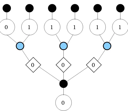
Letv0=u1. . . u2p ∈ U∗ and (t,e)∈TM such thatv0 ∈t1. We definek=k(v0,t) andl=l(v0,t)
in the following way. Write ξ = #t−1 and u0, u1, . . . , u2ξ for the search-depth sequence oft.
Then we set
k = min{i∈ {0,1, . . . ,2ξ}:ui =v0},
l = max{i∈ {0,1, . . . ,2ξ}:ui =v0},
which means that k is the time of the first visit of v0 in the evolution of the contour oft and
that l is the time of the last visit ofv0. Note that l ≥k and that l=k if and only ifv0 ∈∂t.
For everys∈[0,2ξ−(l−k)], we set
b
C(v0)(s) =C(k) +C([[k−s]])−2 inf
u∈[k∧[[k−s]],k∨[[k−s]]]C(u),
whereCis the contour function oftand [[k−s]] stands for the unique element of [0,2ξ) such that [[k−s]]−(k−s) = 0 or 2ξ. Then there exists a unique plane treebt(v0) whose contour function is
b
C(v0). Informally,bt(v0) is obtained fromtby removing all vertices that are descendants ofv
0, by
re-rooting the resulting tree atv0, and finally by reversing the planar orientation. Furthermore
we see that bv0 = 1u2p. . . u2 belongs tobt(v0). In fact, bv0 is the vertex of bt(v0) corresponding to
the root of the initial tree. At last notice thatc∅(bt(v0)) = 1. We now define the functionbe(v0). To this end, foru∈[[∅, v
0]]\ {v0}, letj(u, v0)∈ {1, . . . , cu(t)}
be such thatuj(u, v0)∈[[∅, v0]]. Then set
[[∅, v0]]32 =
u∈[[∅, v0]]∩t3 :e(uj(u, v0)) = 2
[[∅, v0]]41 =
u∈[[∅, v0]]∩t4 :e(uj(u, v0)) = 1 .
For every u ∈bt(v0), we denote by u the vertex which corresponds to u in the treet. We then
setbe(v0)(u) =e(u), except in the following cases :
Sincev0∈t1 we have #[[∅, v0]]32= #[[∅, v0]]41. Indeed, if 1 =e0, e1, . . . , e2p = 1 is the sequence of
types of elements of [[∅, v0]] listed according to their generations, then this list is a concatenation
of patterns of the form 13241, where by 24 we mean an arbitrary (possibly empty) repetition of the pattern 24. If at least one 24 occurs then the second and antepenultimate element of the pattern 13241 correspond respectively to exactly one element of [[∅, v0]]32 and [[∅, v0]]41, while no
term of a pattern 131 corresponds to such elements.
Notice that if (bt(v0),be(v0)) = (T,e), then (t(v0),e(v0)) = (Tb(bv0),be(vb0)). Moreover, if u ∈ T \
{∅,bv0} then we have cu(T) = cu(Tb(vb0)). Recall that if w = (w1, . . . , wn) we write ←w− =
(wn, . . . , w1). To be more accurate, it holds that wu(T) = ←w−u(Tb(bv0)) except in the following
cases :
ifu∈[[∅, v0]]\([[∅, v0]]32∩[[∅, v0]]14) thenwu(T) =←w−uj(u,v0),e(u)(Tb(bv0)),
ifu∈[[∅, v0]]32 thenwu(T) =←w−j(u,vu 0),1(Tb(vb0)),
ifu∈[[∅, v0]]41 thenwu(T) =←w−j(u,vu 0),2(Tb(vb0)),
(2)
where forw∈ W,n=|w|, and 1≤j≤n, we set
wj,1= (wj+1, . . . , wn,1, w1, . . . , wj−1),
wj,2= (wj+1, . . . , wn,2, w1, . . . , wj−1).
In particular, if u ∈ [[∅, v0]]32 (resp. [[∅, v0]]41) with p(wu(Tb(bv0))) = (k, k′,0,0) then
p(wu(T)) = (k+ 1, k′ −1,0,0) (resp. (k −1, k′ + 1,0,0)), while p(wu(Tb(bv0))) = p(wu(T))
otherwise.
Recall the definition of the probability measureQµ.
Lemma 3.4. Let v0 ∈ U∗ be of the form v0 = 1u2. . . u2p for some p∈N. Assume that
Qµ v0∈t1>0.
Then the law of the re-rooted multitype tree(bt(v0),be(v0))underQ
µ(· |v0 ∈t1)coincides with the
law of the multitype tree (t(bv0),e(bv0)) underQ
µ(· |bv0∈t1).
Proof: Let (T,e)∈TM such that bv0 ∈∂1T. We have
Qµ
(bt(v0),be(v0)) = (T,e)=Q µ
(t(v0),e(v0)) = (Tb(bv0),be(bv0)).
And
Qµ
(t(v0),e(v0)) = (Tb(vb0),be(bv0))= Y
u∈Tb(bv0)\{∅,v
0}
ζ(be(bv0)(u))(wu(Tb(bv0))),
Qµ
(t(bv0),e(bv0)) = (T,e)
= Y
u∈T \{∅,vb0}
ζ(e(u))(wu(T)).
[[∅, v0]]41, we obtain
To conclude the proof we use (3) to get that
Qµ(v0 ∈t) =
its offspring is left unchanged by the re-rooting, meaning that
b
ℓui(v0)−bℓu(v0),1≤i≤n=ℓui(vb0)−ℓu(bv0),1≤i≤n.
Otherwise, if u∈[[∅, v0]], setj=j(u, v0), and define the mapping
φn,j : (x1, . . . , xn)7→(xj−1−xj, . . . , x1−xj,−xj, xn−xj, . . . , xj+1−xj).
Then observe that the spatial displacements are affected in the following way:
If (t,e,ℓ)∈TM andw0∈t, we also consider the multitype spatial tree (t(w0),e(w0),ℓ(w0)) where
ℓ(w0) is the restriction ofℓ to the tree t(w0).
Recall the definition of the probability measureQµ,←→ν.
Lemma 3.5. Let v0 ∈ U∗ be of the form v0 = 1u2. . . u2p for some p∈N. Assume that
Qµ v0∈t1>0.
Then the law of the re-rooted multitype spatial tree(bt(v0),be(v0),bℓ(v0))under the measureQ µ,←→ν(· |
v0∈t1) coincides with the law of the multitype spatial tree (t(bv0),e(bv0),ℓ(bv0)) under the measure
Qµ,←→ν(· |bv0 ∈t1).
This lemma is a simple consequence of Lemma 3.4 and our observations around (4) on the spatial displacements ←→ν , combined with the discussion of how the set of children of various vertices are affected by re-rooting, see (1) and (2).
Lemma 3.6. Let w∈ W such thatp3(w) =p4(w) = 0. Setn=|w| and let j∈ {1, . . . , n}.
(i) The image of the measure ←→ν 3,w under the mappingφn,j is
(a) the measure ←→ν 3,wj,1 ifwj = 1,
(b) the measure←→ν 4,wj,2 ifwj = 2.
(ii) The image of the measure ←→ν 4,w under the mappingφn,j is
(a) the measure ←→ν 3,wj,1 ifwj = 1,
(b) the measure←→ν 4,wj,2 ifwj = 2.
Proof: We first suppose that wj = 1. Set k = p1(w), k′ = p2(w) and w0 = 1. Define
e
φn,j = Sn◦φn,j, where as before Sn stands for the mapping (x1, . . . , xn) 7→ (xn, . . . , x1). We
consider a uniform vector (Xl+✶{wl−1=1},1 ≤l ≤n+ 1) on the set Ak,k′ and we set X
(j) =
(Xj+1, . . . , Xn+1, X1, . . . , Xj). Sincew0 =wj = 1, the vector
Xl(j)+✶{wj,1
l−1=1},1≤l≤n+ 1
is uniformly distributed on the setAk,k′ and the measureν3,wj,1 is the law of the vector
X1(j), X1(j)+X2(j), . . . , X1(j)+. . .+Xn(j).
Furthermore we notice thatX1+X2+. . .+Xn+1= 0. This implies that
X1(j), X1(j)+X2(j), . . . , X1(j)+. . .+Xn(j)=φen,j(X1, X1+X2, . . . , X1+. . .+Xn),
which means that the measure ν3,wj,1 is the image of ν3,w under the mapping φen,j. Since
e
φn,j◦Sn=Sn◦φn,n−j+1, we obtain together with what precedes that the measure←−ν3,←w−n−j+1,1 is the image of ←−ν3,←w− under the mapping φen,j. Thus ←→ν 3,wj,1 is the image of ←→ν 3,w under the
action of Sn. Thus we get the first part of the lemma. The other assertions can be proved in
We also denote byvm the first element of ∆1 in the lexicographical order.
The following two Lemmas can be proved from Lemma 3.5 in the same way as Lemma 3.3 and Lemma 3.4 in [9].
Lemma 3.7. For any nonnegative measurable functional F onTM,
Qµ,←→ν
Lemma 3.8. For any nonnegative measurable functional F onTM,
Qµ,←→ν
3.2 Estimates for the probability of staying on the positive side
In this section we will derive upper and lower bounds for the probability Pn
µ,←→ν,x(ℓ > 0) as
n→ ∞. We first state a lemma which is a direct consequence of Lemma 6 in [16].
Lemma 3.9. There exist two constants c0>0 andc1>0 such that
We now establish a preliminary estimate concerning the number of leaves of type 1 in a tree withnvertices of type 1. Write0 for the origin ofR4.
Lemma 3.10. There exists a constant β >0 such that for all nsufficiently large,
Pµ
be the younger brothers of v(n, k) listed in lexicographical order. Here younger brothers are those brothers which have not yet been visited at timenin search-depth sequence. Then we set
ifm≥1 andRn(k) =∅ifm= 0. For everyk >|v(n)|, we setRn(k) =∅. By abuse of notations
we assimilateRnwith (Rn(1), . . . , Rn(|v(n)|)) and letRn=∅if|v(n)|= 0. Standard arguments
(see e.g. [11] for similar results) show that (Rn,e(v(n)),|v(n)|)0≤n≤ξ has the same distribution
as (R′n, e′n, h′n)0≤n≤T′−1, where (R′n, e′n, h′n)n≥0 is a Markov chain starting at (∅,1,0), whose transition probabilities are specified as follows :
• ((r1, . . . ,rh), i, h)→((r1, . . . ,rh,r+h+1),rh+1(1), h+ 1) with probabilityζ(i)({rh+1}) where
r+h+1 = (rh+1(2), . . . ,rh+1(|rh+1|)), for rh+1 ∈ W4\ {∅}, i∈ {1,2,3,4}, r1, . . . ,rh ∈ W4
and h≥0,
• ((r1, . . . ,rh), i, h)→((r1, . . . ,rk−1,r+k),rk(1), k) with probabilityζ(i)({∅}),wheneverh≥
1 and{m≥ 1 :rm 6=∅} 6=∅, and where k = sup{m ≥1 : rm 6=∅}, for i∈ {1,2,3,4},
r1, . . . ,rh∈ W4,
• ((∅, . . . ,∅), i, h)→(∅,1,0) with probability ζ(i)({∅}) for i∈ {1,2,3,4}and h≥0,
and finally
T′ = infn≥1 :h′n= 0 .
WriteP′for the probability measure under which (R′n, en′ , h′n)n≥0is defined. We define a sequence
of stopping times (τj′)j≥0 byτ0′ = 0 andτj+1′ = inf{n > τj′ :e′n= 1}for every j≥0. At last we
set for every j≥0,
Xj′ =✶nhτ′
j+1 ≤hτj′
o
.
Thus we have,
Pµ
|#∂1t−µ(1)({0})n|> n3/4,#t1=n
= P′
nX−1
j=0
Xj′ −µ(1)({0})n> n3/4, τn′−1 < T′ ≤τn′
≤ P′
nX−1
j=0
Xj′ −µ(1)({0})n> n3/4
.
Thanks to the strong Markov property, under the probability measure P′(· | e′
0 = 1), the
random variables Xj′ are independent and distributed according to the Bernoulli distribution with parameter ζ(1)({∅}) = µ(1)({0}). So we get the result using a standard moderate
deviations inequality and Lemma 3.9.
We will now state a lemma which plays a crucial role in the proof of the main result of this section. To this end, recall the definition of vm and the definition of the probability measure
Qnµ
,←→ν.
Lemma 3.11. There exists a constant c >0 such that for all nsufficiently large,
Qnµ
0 0
0 0
0 1
0 0
1
0
0 1 1 1 1
0
Figure 2: The events F (left) and Γ for k= 2 (right)
Proof: We first treat the case where q2k+1 = 0 for every k ≥ 2 which implies that q3 > 0.
Consider the event
E =nz∅(t) = (0,0,1,0),z1(t) = (0,1,0,0),z11(t) = (0,0,0,1),z111(t) = (0,2,0,0),
z1111(t) =z1112(t) = (0,0,0,1),z11111(t) =z11121(t) = (1,0,0,0),
z111111(t) =z111211(t) = (0,0,1,0)
o
.
Let u ∈ U and let (t,e,ℓ) ∈ TM such that u ∈ t. We set t[u] = {v ∈ U : uv ∈ t} and for every v ∈ t[u] we set e[u](v) = e(uv) and ℓ[u](v) = ℓ(uv)−ℓ(u). On the event E we can define (t1,e1,ℓ1) = (t[u1],e[u1],ℓ[u1]) and (t2,e2,ℓ2) = (t[u2],e[u2],ℓ[u2]), where we have written
u1 = 111111 andu2 = 111211. LetF be the event defined by
F =E ∩ nℓ1=ℓ11=ℓ111 =ℓ1111=ℓ1112 =ℓ11111=ℓ11121=ℓ111111 = 0,ℓ111211= 1
o
.
We observe that Qµ,←→ν(F) > 0 and that under Qµ,←→ν(· | F), the spatial trees (t1,e1,ℓ1) and
(t2,e2,ℓ2) are independent and distributed according to Qµ,←→ν. Furthermore
#t1 =n, vm ∈∂1t ⊃F∩ {vm,1 ∈∂1t1} ∩ {ℓ2 ≥0} ∩
#t11+ #t12 =n−1 ,
wherevm,1 is the first vertex of t11\ {∅}that achieves the minimum of ℓ1. So we obtain that
Qµ,←→ν #t1=n, vm∈∂1t (5)
≥ Qµ,←→ν(F)
nX−2
j=1
Qµ,←→ν #t1=j, vm∈∂1t
Let us now turn to the second case for which there exists k ≥ 2 such that q2k+1 > 0. Let
We can now conclude the proof of Lemma 3.11 in both cases from respectively (5) and (6) by following the lines of the proof of Lemma 4.3 in [9].
We can now state the main result of this section.
Proposition 3.12. Let M >0. There exist four constants γ1 >0, γ2 >0, eγ1 >0 and γe2 >0
such that for all n sufficiently large and for every x∈[0, M],
e
Proof: We prove exactly in the same way as in [9] the existence of eγ2 and the existence of a
constantγ3 >0 such that for all nsufficiently large, we have
Let us now fix M > 0. Let k ≥ 1 be such that q2k+1 > 0. We choose an integer p such
that pk ≥ M. First note that ←→ν 3,w({0}) = 1/(2k −1) if w = (0,2k−1,0,0) and that
←→ν
4,w({k, k−1, . . . ,1}) = 1/(2#Ak,0) if w = (k,0,0,0). For every l ∈N, we define 1l ∈ U by
1l= 11. . .1, |1l|=l. By arguing on the event
E′ =nz∅(t) =. . .=z14p(t) = (0,0,1,0),z1(t) =. . .=z14p−3(t) = (0,2k−1,0,0), z11(t) =. . .=z1(2k−1)(t) =. . .=z14p−31(t) =. . .=z14p−3(2k−1) = (0,0,0,1), z111(t) =. . .=z1(2k−1)1(t) =. . .=z14p−311(t) =. . .=z14p−3(2k−1)1= (k,0,0,0)
o
∩
p\−1
i=0
{z14i+32(t) =. . .=z14i+3k=0} ∩
p\−1
i=0 2k\−1
j=2 k
\
l=1
{z14i+1j1l=0},
we show that
Qµ,←→ν ℓ>0,#t1=n ≥ C(µ,ν, k)
p
µ(1)({(0,0,1,0)})Pµ,←→ν,pk ℓ>0,#t1 =n−pk(2k−1)
,
whereC(µ,ν, k) is equal to
µ(1)({(0,0,1,0)})µ(3)({(0,2k−1,0,0)})(µ(4)({(k,0,0,0)}))2k−1µ(1)({0}))k(2k−1)−1
(2k−1)(2#Ak,0)2k−1
.
This implies thanks to Lemma 3.9 that for all nsufficiently large,
Pnµ,←→ν,pk(ℓ>0)≤ 2µ
(1)({(0,0,1,0)})eγ 2
C(µ,ν, k)n ,
which ensures the existence ofγ2.
Last by arguing on the event
F =nz∅(t) =z14 = (0,0,1,0),z1(t) = (0,2k−1,0,0),
z11(t) =. . .=z1(2k−1)(t) = (0,0,0,1),z111(t) =. . .=z1(2k−1)1(t) = (k,0,0,0)
o
∩
k
\
j=2
{z13j(t) =0} ∩
2k\−1
i=2 k
\
j=1
{z1i1j(t) =0},
we show that
Pµ,←→ν,0 ℓ>0,#t1 =n
≥ C(µ,ν, k)µ(1)({(0,0,1,0)})Qµ,←→ν ℓ≥0,#t1 =n−k(2k−1),
3.3 Proof of Theorem 3.3
To prove Theorem 3.3 from what precedes, we can adapt section 7 of [9] in exactly the same way as in the proof of Theorem 3.3 in [19]. A key result in the proof of Theorems 2.2 in [9] and 3.3 in [19] is a spatial Markov property for spatial Galton-Watson trees. Let a > 0 and (t,e,ℓ) ∈TM. As in section 5 of [9] letv1, . . . , vM denote the exit vertices from (−∞, a) listed
in lexicographical order, and let (ta,ea,ℓa) correspond to the multitype spatial tree (t,e,ℓ) which has been truncated at the first exit from (−∞, a). Let v∈t. Recall from section 3.2 the definition of the multitype spatial tree (t[v],e[v],ℓ[v]). We set ℓ[v]u =ℓ[v]u +ℓv for everyu∈t[v].
Lemma 3.13. Let x ∈[0, a) and p ∈ {1, . . . , n}. Let n1, . . . , np be positive integers such that
n1+. . .+np≤n. Assume that
P(1),nµ
,←→ν,x
M =p, #t[v1],1 =n
1, . . . , #t[vp],1 =np
>0.
Then, under the probability measure P(1),nµ,ν,x(· | M = p, #t[v1],1 = n
1, . . . ,#t[vp],1 = np), and
conditionally on (ta,ea,ℓa), the spatial trees
t[v1],e[v1],ℓ[v1], . . . ,t[vp],e[vp],ℓ[vp]
are independent and distributed respectively according to P(e(v1)),n1
µ,←→ν,ℓv1 , . . . ,P
(e(vp)),np
µ,←→ν,ℓvp .
Observe that in our context, if v is an exit vertex then e(v) ∈ {1,2}. This is the reason why Theorem 3.3 is stated under both probability measuresP(1),n
µ,←→ν,xandP (2),n
µ,←→ν,x. Thus the statement
of Lemma 7.1 of [9] (and of Lemma 3.18 of [19]) is modified in the following way. Set for every n≥1 and everys∈[0,1],
C(n)(s) = AqC((#t−1)s) n1/2 ,
V(n)(s) = BqV((#t−1)s) n1/4 .
Last define from section 1.2.2, on a suitable probability space (Ω,P), a collection of processes (bx,rx)x>0.
Lemma 3.14. Let F : C([0,1],R)2 → R be a Lipschitz function. Let 0 < c′ < c′′. Then for i∈ {1,2},
sup
c′n1/4≤y≤c′′n1/4
E
(i),n
µ,ν,y
FC(n), V(n)−E
F
bBqy/n1/4
,rBqy/n1/4
n−→→∞0.
4
Proof of Theorem 1.2
set ξ = #t−1 and we denote by v(0) = ∅≺ v(1) ≺. . . ≺v(ξ) the list of the vertices of t in
Note that Kt(k) is the number of vertices of type 1 in the search-depth sequence up to time k. As previously, we extend Kt to the real interval [0,2ξ] by setting Kt(s) =Kt(⌊s⌋) for every s∈[0,2ξ], and we set for everys∈[0,1] mass at the identity mapping of [0,1]. In other words, for every η >0,
P(1),nµ,←→ν,1 sup mass at the identity mapping of [0,1]. In other words, for every η >0,
P(1),nµ,←→ν,1 sup
type 1 in lexicographical order. We define as in [16]
Gt
Thus we obtain thanks to Lemma 3.9 and Proposition 3.12 that for everys∈[0,1], there exists a constantε′ >0 such that for all nsufficiently large,
Let us fixη >0. We then have for everys∈[0,1],
which implies that for every s∈[0,1],
P(1),nµ,←→ν,1 |(#t)−1Gt1(⌊ns⌋)−s| ≥η −→
n→∞0.
Let us now set kη = ⌈a21η⌉ and sm = mkη−1 for every m ∈ {0,1, . . . , kη}. Since the mapping
s∈[0,1]7→n−1Gt
1(⌊ns⌋) is non-decreasing, we have
P(1),nµ,←→ν,1 sup
We can now complete the proof of Theorem 1.2. Recall thatRm denotes the radius of the map
m. Thanks to Proposition 2.1 we know that the law ofRm under Brq(· | #Vm =n) coincides
Let us turn to (ii). By Proposition 2.1 and property (ii) of the Bouttier-Di Francesco-Guitter bijection stated at the end of Section 2.3, the law of λ(n)m under Brq(· | #Vm = n) is the law
which coincides with the law ofInunderP (1),n
µ,←→ν,1. We thus complete the proof of (ii) by following
the lines of the proof of Theorem 2.5 in [19]. Finally, assertion (iii) easily follows from (ii).
[2] Ambjørn, J., Durhuus, B., Jonsson, T. (1997) Quantum geometry. A statistical field theory approach. Cambridge Monographs on Mathematical Physics. Cambridge University Press, Cambridge. MR1465433
[3] Bouttier J., Di Francesco P., Guitter E. (2004) Planar maps as labeled mobiles. Electron. J. Combin. 11, R69 MR2097335
[4] Chassaing, P., Schaeffer, G.(2004) Random planar lattices and integrated superBrow-nian excursion. Probab. Th. Rel. Fields128, 161–212. MR2031225
[5] Cori, R., Vauquelin, B. (1981) Planar maps are well labeled trees.Canad. J. Math. 33, 1023-1042. MR0638363
[6] Gromov, M. (1999) Metric structures for Riemannian and non-Riemannian spaces, vol-ume 152 of Progress in Mathematics. Birkh¨auser Boston Inc., Boston, MA. MR1699320
[7] Le Gall, J.-F. (1999)Spatial Branching Processes, Random Snakes and Partial Differen-tial Equations.Lectures in Mathematics ETH Z¨urich. Birkh¨auser, Boston. MR1714707
[8] Le Gall, J.-F. (2005) Random trees and applications. Probab. Surveys 2, 245–311. MR2203728
[9] Le Gall, J.-F. (2006) A conditional limit theorem for tree-indexed random walk. Stoch. Process. Appl. 116, 539–567. MR2205115
[10] Le Gall, J.-F. (2007) The topological structure of scaling limits of large planar maps. Invent. Math., 169:621–670. MR2336042
[11] Le Gall, J.-F., Le Jan, Y.(1998) Branching processes in L´evy processes : the exploration process. Ann. Probab.26, 213–252. MR1617047
[12] Le Gall, J.-F., Paulin, F.(2006) Scaling limits of bipartite planar maps are homeomor-phic to the 2-sphere. To appear inGeom. Funct. Anal.math/0612315.
[13] Le Gall, J.-F., Weill, M. (2006) Conditioned Brownian trees.Ann. Inst. H. Poincar´e Probab. Statist. 42, 455–489. MR2242956
[14] Marckert, J.-F., Miermont, G.(2007) Invariance principles for random bipartite planar maps. Ann. Probab.35, 1642–1705. MR2349571
[15] Marckert, J.-F., Mokkadem, A. (2006) Limits of normalized quadrangulations. The Brownian map. Ann. Probab. 34, 2144–2202. MR2294979
[16] Miermont, G.(2006) Invariance principles for spatial multitype Galton-Watson trees. To appear in Ann. Inst. H. Poincar´e Probab. Statist.math.PR/0610807
[18] Schaeffer, G.(1998) Conjugaison d’arbres et cartes combinatoires al´eatoires. PhD thesis, Universit´e Bordeaux I.
![Figure 1: The branch leading from ∅ to v0, and the corresponding branch in the tree �t(v0): thebranch is put upside-down and the vertices of [[∅, v0]]32 and [[∅, v0]]41 interchange their roles.](https://thumb-ap.123doks.com/thumbv2/123dok/980206.915824/16.612.168.430.81.377/figure-branch-leading-corresponding-branch-thebranch-vertices-interchange.webp)