KREIN SPACES NUMERICAL RANGES AND
THEIR COMPUTER GENERATION∗
N. BEBIANO†, J. DA PROVIDˆENCIA‡, A. NATA§, AND G. SOARES¶
Abstract. LetJbe an involutive Hermitian matrix with signature (t, n−t), 0≤t≤n,that is, withtpositive andn−tnegative eigenvalues. The Krein space numerical range of a complex matrix
Aof sizenis the collection of complex numbers of the form ξξ∗∗J AξJ ξ , withξ∈C
nandξ∗J ξ= 0. In this note, a class of tridiagonal matrices with hyperbolical numerical range is investigated. AMatlab program is developed to generate Krein spaces numerical ranges in the finite dimensional case.
Key words. Krein spaces, Numerical range, Tridiagonal matrices.
AMS subject classifications.15A60, 15A63.
1. Introduction. Throughout, Mn denotes the algebra of n×nmatrices over the field of complex numbers. LetJbe an involutive Hermitian matrix with signature (t, n−t), 0≤t≤n,that is, withtpositive andn−tnegative eigenvalues. ConsiderCn
as a Krein space with respect to the indefinite inner product [ξ, η] =η∗Jξ, ξ, η∈Cn.
TheJ−numerical range ofA∈Mn is denoted and defined by:
WJ(A) =
[Aξ, ξ]
[ξ, ξ] : ξ∈C
n, [ξ, ξ]
= 0
.
Considering J the identity matrix of order n, In, this concept reduces to the well knownclassical numerical range, usually denoted byW(A). The numerical range of an operator defined on an indefinite inner product space is currently being studied (see [11] and references therein). ForWJ(A),A∈Mn, the following inclusion holds:
σ(A)⊂WJ(A), whereσ(A) denotes the set of the eigenvalues ofAwithJ−anisotropic eigenvectors, that is, eigenvectors with nonvanishingJ−norm. We denote byσ±(A) the sets of the eigenvalues ofA with associated eigenvectorsξsuch that ξ∗Jξ=±1. Compactness and convexity are basic properties of the classical numerical range. In
∗Received by the editors December 17, 2007. Accepted for publication March 24, 2008. Handling Editor: Peter Lancaster.
†CMUC, Department of Mathematics, University of Coimbra, Coimbra, Portugal ([email protected]).
‡CFT, Department of Physics, University of Coimbra, Coimbra, Portugal ([email protected]).
§CMUC, Department of Mathematics, Polytechnic Institute of Tomar, Tomar, Portugal ([email protected]).
¶Department of Mathematics, University of Tr´as-os-Montes and Alto Douro, Vila Real, Portugal ([email protected]).
contrast with the classical case, WJ(A) may be neither closed nor bounded. On the other hand, WJ(A) may not be convex, but it is the union of two convex sets
WJ(A) =WJ+(A)∪WJ−(A),where
WJ+(A) =
[Aξ, ξ]
[ξ, ξ] : ξ∈C
n, [ξ, ξ]>0
and
WJ−(A) =
[Aξ, ξ]
[ξ, ξ] : ξ∈C
n, [ξ, ξ]<0
.
Since the Krein space numerical range is in general neither bounded nor closed, it is difficult to generate an accurate computer plot of this set. For A∈Mn andn >2, the description of WJ(A) is complicated, and so it is of interest to have a code to produce graphical representations. The case n = 2 is treated by the Hyperbolical Range Theorem [1] which states the following: ifA∈M2has eigenvaluesα1andα2,
J = diag(1,−1) and 2Re (α1α2) < Tr(A[∗]A) < |α1|2+|α2|2, where A[∗] = JA∗J, then WJ(A) is bounded by a nondegenerate hyperbola with foci at α1 andα2, and transverse and nontransverse axis of length
Tr(A[∗]A)−2Re (α1α2¯) and |α1|2+|α2|2−Tr(A[∗]A),
respectively. For the degenerate cases, WJ(A) may be a singleton, a line, the union of two half-lines, the whole complex plane, or the complex plane except a line. Inde-pendently of the size, certain matrices have a hyperbolicalJ−numerical range.
A matrixA= (aij)∈Mnistridiagonalifaij = 0 whenever|i−j|>1.Interesting papers have been published on the classical numerical range of tridiagonal matrices [3, 4, 12]. For complex numbers a, b, c, the tridiagonal matrix in Mn with a′s on the main diagonal, b′s on the first superdiagonal and c′s on the first subdiagonal is denoted byA = tridiag(c, a, b). These matrices are ofToeplitz type, because all the entries in each diagonal are equal. Marcus and Shure [12] proved that the numerical range of tridiag(0,0,1) is a circular disc centered at the origin of radius cos(π/(n+1)). Eiermann [6] showed that the numerical range of tridiag(c,0, b) is the elliptical disc {cz+bz : |z| ≤cos(π/(n+ 1))}.Generalizations of Eiermann’s results were given by Chien [3, 4], Chien and Nakazato [5], and Brown and Spitkovsky [2]. Likewise, there is interest in studying Krein spaces numerical ranges of these classes.
2. A class of tridiagonal matrices with hyperbolical numerical range. The proof of the next lemma is similar to the proof of Lemma 3.1 in [2] and is included for the sake of completeness.
Lemma 2.1. LetJ beI1⊕ −I1⊕ · · · ⊕I1⊕ −I1⊕I1 orI1⊕ −I1⊕ · · · ⊕I1⊕ −I1
according to the size of the matrixJ being odd or even, respectively. TheJ−numerical range of an n×n tridiagonal matrix is invariant under interchange of the (j, j+ 1) and(j+ 1, j)entries for anyj = 1, . . . , n−1.
Proof. Let
A=
a1 b1 0 · · · 0
c1 . .. ... ... ...
0 . .. aj bj . .. ... ..
. . .. cj aj+1 . .. 0 ..
. . .. ... . .. bn−1
0 · · · 0 cn−1 an
.
(2.1)
For simplicity we interchangeb1 and c1.Let ˆA be the n×n tridiagonal matrix that differs from A only by interchanging b1 and c1. Consider an arbitrary point z =
z∗JAz ∈WJ(A), where z = (z1, . . . , zn)T ∈Cn and z∗Jz = 1. We show that there exists ˆz= (ˆz1, . . . ,znˆ )T ∈Cn such thatz∗JAz= ˆz∗JAˆzˆand z∗Jz= ˆz∗Jzˆ. For the first equality to hold, we require that
¯
z1a1z1−z2a2z2¯ + ¯z1b1z2−z2c1z1¯ = ¯ˆz1a1z1ˆ −¯ˆz2a2z2ˆ + ¯ˆz1c1z2ˆ −¯ˆz2b1z1.ˆ
If z1 = 0, we can choose ˆz = z. Otherwise, let |z1ˆ | = |z1|, |z2ˆ | = |z2|, arg ˆz1 = −argz1+π, arg ˆz2 = −argz2. Moreover, we choose ˆzj =zjeiφ, j >2, where φ =
−2 argzj.By easy calculations, the result follows.
A supporting line of a convex set S ⊂C is a line containing a boundary point
of S and defining two half-planes, such that one of them does not contain S. The supporting lines ofWJ(A) are by definition the supporting lines of the convex sets
WJ+(A) andWJ−(A). Let
HA=A+A
[∗]
2 and KA=
A−A[∗]
2i .
(2.2)
be the unique J−Hermitian matrices such that A = HA+iKA. (A matrix A is
J−Hermitian if it coincides with A[∗].) If ux+vy+w = 0 is the equation of a
We recall thatA∈Mn is essentiallyJ−Hermitianif there exist ζ1, ζ2∈Csuch
that A = ζ1In +ζ2A′ where A′ is J−Hermitian. In this case, WJ(A) is a line or the union of two half-lines [13]. Next, we assume that A ∈ Mn is nonessentially
J−Hermitian.
Theorem 2.2. LetA∈Mn be a nonessentiallyJ−Hermitian tridiagonal matrix
with biperiodic main diagonal, that is, aj =a1 if j is odd and aj =a2 if j is even, and with off-diagonal entries bj, cj such that either cj = kbj or bj =kcj for some
k∈Candj = 1, . . . , n−1. LetJ be the diagonal matrixI1⊕ −I1⊕ · · · ⊕I1⊕ −I1⊕I1
or I1 ⊕ −I1 ⊕ · · · ⊕I1 ⊕ −I1 according to the size of A being odd or even. Let
γ = (a1−a2
2 )2+kλ21, where λ1 is the spectral norm of C = tridiag (c,0,b)∈Mn for
0= (0,0, . . . ,0),b= (b1,−b2, . . .)andc= (b1,−b2, . . .). The following holds:
(i) If |γ| > 12λ2
1(1 +|k|2)−
a1−2a2
2
, then WJ(A) is bounded by the hyperbola centered at a1+a2
2 , foci at
(a1+a2)±(a1−a2)2+ 4kλ2 1
2
and semi-transverse axis of length
α=
1 2
a1−a2
2
2
−1
4λ
2
1(1 +|k|2) +
1 2|γ|.
(ii) If |γ|= 12λ2
1(1 +|k|2)−
a1−2a2
2
, then WJ(A) is the whole complex plane except the line with slope (arg(γ) +π)/2passing through (a1+a2)/2.
(iii) If|γ|< 12λ2
1(1 +|k|2)−
a1−2a2
2
, thenWJ(A) is the whole complex plane.
Proof. LetA have even size. According to Lemma 2.1, we may assume without loss of generality that the off-diagonal entries of A are such that cj =kbj, for j = 1, . . . , n−1. Writingc= (a1−a2)/2, we haveA= 12(a1+a2)In+B, where the matrix
B is obtained fromAreplacing the main diagonal by (c,−c, . . . , c,−c). Without loss of generality, we may assume thatc >0.
det (Re (e−iθJB)−µ(θ)J) = 2−n|e−iθ−keiθ|n ×det
Re (c e−iθ )−µ(θ)
1/2|e−iθ−keiθ| b1 0 · · · 0
b1 Re (c e− iθ
)+µ(θ) 1/2|e−iθ
−keiθ
| −b2 . ..
.. .
0 −b2 Re (c e−
iθ )−µ(θ) 1/2|e−iθ
−keiθ
| . .. 0
..
. . .. . .. . .. bn−1
0 · · · 0 bn−1 Re (c e
−iθ )−µ(θ) 1/2|e−iθ−keiθ|
.
For (Re (c e−
iθ
))2−µ(θ)2 1/4|e−iθ−keiθ|2 =λ
2, the determinant in the right hand side of the above
equality coincides with the determinant ofC−λIn, whereC is the tridiagonal Her-mitian matrix with vanishing main diagonal, first superdiagonal and subdiagonal (b1,−b2, . . . , b1) and (b1,−b2, . . . , b1), respectively. The eigenvalues of the Hermitian matrixCoccur in pairs of symmetric real numbers, and we denote and order them as follows: λ1>· · ·> λn
2 >· · ·> λn, withλn−j+1=−λj, j= 1, . . . , n. The eigenvalues
ofJRe (e−iθJB), sayµj(θ), satisfy
µ2j(θ) = (Re (c e−iθ))2− λ2
j
4 |e −iθ
−keiθ|2∈R, j = 1, . . . , n.
(2.3)
Letθ be fixed but arbitrary. We analyze the condition for the eigenvaluesµj(θ) to be real. If the smallest of the µ2
j(θ), that is, µ21(θ), is nonnegative, then all the µj(θ) are real. So, we investigate the existence of anglesθsuch that
µ21(θ) =P+Qcos(2θ) +Rsin(2θ)≥0,
where
P =1 2c
2
−14λ21(1 +|k|2),
Q=1 2Re (c
2) +1
2Re (k)λ
2 1, R=1
2Im(c
2) +1
2Im(k)λ
2 1.
Writingγ= 2(Q+iR) =c2+kλ2
1 and Γ = arg(γ), we have
µ21(θ) =αcos2
Γ 2 −θ
−βsin2
Γ 2 −θ
,
where
α= 1 2c
2−1
4λ
2
1(1 +|k|2) +
and
β=−12c2+1 4λ
2
1(1 +|k|2) +
1 2|γ|. (2.4)
We show thatβ ≥0.In fact, since
|γ| 2 ≥
1 2c
2
− |k|λ
2 1
2 ,
from (2.4) we easily conclude that
β ≥1 4λ
2
1(1− |k|)2≥0.
It can be easily seen that a tridiagonal matrixAunder the hypothesis of the theorem is essentially J−Hermitian if and only if |k| = 1 and arg k = 2 argc. Since A is nonessentially J−Hermitian, then |k| = 1 and to avoid trivial situations we may supposeλ1= 0.Thus, we may considerβ >0.
If (i) holds, then |γ|> 1 2λ
2
1(1 +|k|2)−c2, and soα >0. Thus there exist angles θsuch thatµ2
1(θ)≥0.Hence
µ1(θ) =±
αcos2
Γ
2 −θ
−βsin2
Γ
2 −θ
,
(2.5)
and all the µj(θ) are real and pairwise symmetric. It can be easily seen that (2.5) describes a family of hyperbolas, forθ ranging over [θ1, θ2],tan(Γ/2−θi) =α/β, i= 1,2. The parametric equations of the hyperbola generated byµj(θ) are
xcos(θ) +ysin(θ) =µj(θ) −xsin(θ) +ycos(θ) =µ′
j(θ)
for θ ∈ [Γ/2,Γ/2 + 2π[. Since 0 < µ1(θ) < µ2(θ) < · · · < µn
2(θ), these eigenvalues
originate a collection of nested hyperbolas. The outer hyperbola is generated byµ1(θ) and its Cartesian equation is
X2 α −
Y2 β = 1,
(2.6)
whereX =xcos(Γ/2)−ysin(Γ/2) and Y =xsin(Γ/2) +ycos(Γ/2).
Now, we analyze the sign of theJ−norm of the eigenvectors associated withµj(θ). We notice that if νj =x(j)1 , . . . , x(j)n
is an eigenvector associated with µj(θ), then
νn−j+1=
sx(j)1 , x (j) 2 , sx
(j) 3 , . . . , x
(j) n
is an eigenvector associated with−µj(θ),where
s= ccosθ−µj(θ)
Easy calculations show that theJ−norm ofνj is
|x(j)1 |2+|x(j)
3 |2+· · ·+|x(j)n |2
(1−s),
while theJ−norm ofνn−j+1 is
|x(j)1 |2+|x(j)3 |2+· · ·+|x(j)n |2
s(s−1).
Therefore, µj(θ)∈σ+(JRe (e−iθJB)), j = 1, . . . ,n
2 and µn−j+1(θ)∈σ
−(JRe (e−iθ JB)), j= n2+ 1, . . . , n. Hence,
WJ+(JRe (e−iθJB)) = [µ1(θ),+∞[ ; WJ−(JRe (e−iθJB)) = ]− ∞,−µ1(θ)].
(2.7)
Thus,∂WJ(A) is the asserted hyperbola.
Now, we consider thatAhas odd size. The situation is similar to the one treated above, with the eigenvalues ofJRe (e−iθJ B) occurring in pairs of symmetric real
num-bers, being Re (e−iθc) an eigenvalue with associated eigenvector (x(j) 1 ,0, x
(j) 3 , . . . , x
(j) n )
of positiveJ−norm. Forθ= 0, we have
α≤c2−12λ21(1− |k|2).
Therefore,√α≤c, so the point clies inside the hyperbola (2.6). Thus, (i) follows.
(ii) If|γ|= 12λ2
1(1 +|k|2)−c2, then α= 0 andµ21(θ)<0 for all θ = Γ/2. The
matrixJRe (Je−iθB) has complex eigenvalues in all directions, except in the direction θ= Γ/2.Thus, the projection ofWJ(A) in all the directions is the whole line, possibly except in the direction θ= Γ/2. Thus, we may conclude thatWJ(A) is the complex plane possibly without one line. Now, we show that the line with slope (Γ +π)/2 and passing through (a1+a2)/2 is not contained in WJ(A).
Since µ2
1(Γ/2) = 0, 0 is a double eigenvalue ofBΓ/2 :=JRe (Je−iΓ/2B) and we
use a perturbative method. LetBǫΓ/2=JRe (e−iΓ/2JBǫ),whereBǫ is obtained from Breplacingcbyc+ǫ,withǫ∈Rchosen as follows. We haveα(ǫ) =α+ǫ M+O(ǫ2),
where M is real and nonzero. Choosing ǫ such that ǫ M is positive, then α(ǫ) >0 and by (2.7), we may conclude that WJ+(B
Γ/2 ǫ ) =
α(ǫ),+∞ and WJ−(B Γ/2 ǫ ) =
−∞,−
α(ǫ). Ifǫ → 0, then α(ǫ) → 0 and we find that ]− ∞,0[ ∪ ]0,+∞[ is
contained inWJ(BΓ/2).
We show that the origin is not an element of WJ(BΓ/2). Firstly, we assume
that n is even and we use a perturbative method. Let the eigenvalues of BǫΓ/2 be µ1(ǫ), . . . , µn/2(ǫ)∈σ+(BΓ/2
ǫ ) andµn/2+1(ǫ), . . . , µn(ǫ)∈σ−(BǫΓ/2) with associated
· · ·< µn/2(ǫ). Consider the basisB(ǫ) obtained from the above eigenbasis replacing the vectors ν1(ǫ) and νn(ǫ), respectively, by v1(ǫ) and vn(ǫ), with J−norms 1 and −1, so that the matrixBΓ/2ǫ is represented inB(ǫ) in the formB1(ǫ)⊕B2(ǫ)⊕B3(ǫ),
whereB1(ǫ) = diag(µn
2(ǫ), . . . , µ2(ǫ)),
B2(ǫ) =
1 1−α2(ǫ)
−
1−α2(ǫ) −1
,
andB3(ǫ) = diag(µn+1(ǫ), . . . , µn/2+1(ǫ)).Clearly,
B2(ǫ) =
1
1−α2(ǫ)
−
1−α2(ǫ) −1
−−→ǫ→0
1 1
−1 −1
.
Taking the limit of each element of B(ǫ) asǫ→0, we obtain the basis denoted by B.
Letv=x1v1+xnvn+
n−1
i=2
xiνi be an arbitrary anisotropic vector ofCn expressed in
B.So
v∗JBv
v∗Jv =
|x1+xn|2+µ2(|x2|2+|xn
−1|2) +· · ·+µn 2(|x
n 2|
2+|x2n 2+1|)
|x1|2− |xn|2+|x2|2− |xn
−1|2+· · ·+|xn 2|
2− |xn 2+1|
2 ∈W
+ J(BΓ/2).
Sincevis anisotropic, the denominator is nonzero and the numerator vanishes if and only ifx2=xn−1=· · ·=xn
2 =x n
2+1= 0 andxn+x1= 0,which is impossible. Ifn
is odd an analogous argument holds.
(iii) If |γ| < 12λ21(1 +|k|2)− |c|2, then µ21(θ) is negative and so µ1(θ) is
imagi-nary. Thus, the projection of WJ(A) in each direction is the whole line, and as a consequence,WJ(A) =C.
Corollary 2.3. Let J be the infinite diagonal matrixI1⊕ −I1⊕ · · ·and let A
be the infinite tridiagonal matrix with biperiodic main diagonal, that is,aj =a1 if j
is odd and aj =a2 if j is even, and with off-diagonal entriesbj, cj such that either
cj =kbj orbj=kcj k∈C,j = 1,2, . . .. Letγ= (a1−a2
2 )2+k(|b1|+|b2|)2. Then:
(i) If |γ| > 12(|b1|+|b2|)2(1 +|k|2)− a1−2a2
2
, then WJ(A) is the open region bounded by the hyperbola centered at a1+a2
2 , foci at
(a1+a2)±
(a1−a2)2+ 4k(|b1|+|b2|)2
2
and semi-transverse axis of length
1 2
a1−a2
2 2
−14(|b1|+|b2|)2(1 +|k|2) +1
(ii) If|γ|= 1
2(|b1|+|b2|)
2(1 +|k|2)− a1−2a2
2
, thenWJ(A)is the whole complex plane except the line with slope arg(γ)+π2 passing through a1+a2
2 .
(iii) If|γ|< 1
2(|b1|+|b2|)
2(1 +|k|2)− a1−2a2
2
, thenWJ(A)is the whole complex plane.
Proof. The corollary is a simple consequence of the last theorem, by taking limits as the size of A∈Mn tends to infinity. Having in mind that the eigenvalues of the matrixC∈Mn in Theorem 2.2 are (cfr. [8])
λ= 0 and λr=±
|b1|2+|b2|2+ 2|b1||b2|cos
rπ
m+ 1
, r= 1, . . . , m
forn= 2m+ 1 and
λr=±|b1|2+|b2|2+ 2|b1||b2|Qr, r= 1, . . . , m
forn= 2m, whereQr,r= 1, . . . m,are the roots of the polynomialqm(µ) recurrently defined by
q0(µ) = 1, q1(µ) = 1 +β, β2=|b2|
2
|b1|2, qm+1(µ) =µqm(µ)−qm−1(µ), m >1.
Asntends to infinity we can easily show thatλ2
1= (|b1|+|b2|)2.In the infinite case,
the half-rays (2.7) are open. In fact, if their origins were attained, they would be eigenvalues of the infinite matrixJRe (e−iθJB), which is impossible since under the
hypothesis the matrix is non scalar. Thus,WJ(A) is the open region bounded by the asserted hyperbola in (i). Now, the corollary straightforwardly follows.
Remark 2.4. Given A =HA+i KA ∈ Mn, with HA and KA as in (2.2), the
J−generalized Levinger transformofA (see [7]) is defined by
LJ(A, α, β) =αHA+βKA, with α, β∈R.
For everyα, β∈R, we clearly have
HL(A,α,β)=αHA and KL(A,α,β)=−iβKA.
Thus, we may write
WJ(LJ(A, α, β)) ={α x+i β y: x, y∈R, x+i y∈WJ(A)}.
There is a relation between WJ(A) and WJ(LJ(A, α, β)), in case the sets are
hy-perbolical. In fact, supposing that the boundary of WJ(A) in the plane (u, v) has equation
u2 M2 −
v2
for α = 0 and β > 0, changing the variables u = α−1X and v = β−1Y, then the
boundary ofWJ(A) is the hyperbola
X2 α2M2 −
Y2 β2N2 = 1.
3. Algorithm and Examples. As an heuristic tool, it is convenient to have a code to produce the plot ofWJ(A). In [10], aMatlab program for plotting WJ+(A),
A∈Mn,was presented and the authors mention that there is place to improvement. We would like to observe that in some cases, such as in Example 3.4 (Figure 3.3), this program fails. We include aMatlabprogram to generate Krein spaces numerical ranges of arbitrary complex matrices that treats the degenerate cases and represents the boundary generating curves. As an essential complement, an algorithm is given for computing the pseudoconvex hull of a finite number of points. The accuracy of our program is quite good because a routine, namelyrounding.m, was implemented to remove the rounding errors in the program. Its speed is equivalent to the one of the program in [10]. We emphazise that our program plots the boundary generating curves and their pseudoconvex hull. Moreover, it also works for Hilbert spaces numerical ranges.
Our approach uses the elementary idea that the boundary, ∂WJ(A) , may be traced by computing the extreme eigenvalues (as specified below) of
JRe
e−iθJA
in σ+(JRe
e−iθJA
) and in σ−(JRe
e−iθJA
), and the associated eigenvectors νθ+ and νθ−, for θ running over a finite discretization of 0≤θ < π. The points
νθ+∗JAν+θ νθ+∗Jνθ+ and
νθ−∗JAν−θ νθ−∗Jνθ−
are boundary points ofWJ+(A) andWJ−(A), respectively.
To describe the algorithm, we recall the concepts of noninterlacing eigenvalues and of pseudoconvex hull of a set of points.
Let H be aJ−Hermitian matrix whose eigenvalues are all real and α1 ≥ · · · ≥
αr∈σ+(H) and αr+1 ≥ · · · ≥αn ∈σ−(H). If αr > αr+1 or αn > α1,we say that the eigenvalues ofH do not interlace.
Consider a set of pointsP ={p1, . . . , pk} ⊂Rk with associated signs{ǫ1, . . . , ǫk},
where ǫj =±1, j = 1, . . . , k. The pseudoconvex hull of P is the set of the pseudo convexcombinations of points, that is, the set of the form
k
j=1tjǫjpj
k
j=1ǫjtj
:tj≥0, j= 1,2, . . . , k, k
j=1
ǫjtj= 0
If theǫj are all equal, then the pseudoconvex hull reduces to the convex hull.
Step 1: For an arbitrary complex matrixAof ordern, compute the eigenvalues of the matrixJRe
e−iθrJA, with
θr=π(r−1)
2m , r= 1, . . . ,2m
for some positive integerm and for some involutive Hermitian matrixJ. Construct the vector formed by all the values ofrsuch that the matrixJRe
e−iθrJAhas at
least one real eigenvalue. For each choice ofr, test the multiplicity of the eigenvalues. If there exists at least one multiple eigenvalue, perturb the directionθr. If the above mentioned vector is nonempty and there exists at least a value of r such that the eigenvalues of the matrix JRe
e−iθrJA are all real with anisotropic eigenvectors,
go to Step 2. Otherwise, go to Step 5 and we have a degenerate case.
Step 2: For each θr described above, compute the eigenvalues of the matrix
JRe
e−iθrJA, and the associated eigenvectorsξi(r), i= 1, . . . , n.Evaluate
ρi(r) = ξi(r)
∗JAξi(r)
ξi(r)∗Jξi(r) , i= 1, . . . , n
and construct two vectors formed by the elements ρi(r) such that the sign of the scalar ξi(r)∗Jξi(r) is +1 and −1, respectively. The components of these vectors produce points of the boundary generating curves ofWJ(A).
Step 3: Investigate the existence of directions for which the eigenvalues of the matrixJRe
e−iθrJAdo not interlace. If they exist, go to the next step. Otherwise,
follow to Step 5.
Step 4: Compute the pseudoconvex hull of the boundary generating curves of
WJ(A).
Step 5: Compute ζ ∗
iJAζi ζ∗
iJζi
for a sample of anisotropic vectorsζirandomly chosen.
The distribution of these points allows to conclude whether WJ(A) is the complex plane (possibly the complex plane without a line) or a line (possibly without a point).
Remark 3.1. Obviously, if J = I,−I, then WJ(A) reduces to the classical
numerical range. In this case, the algorithm consists of the Steps 1, 2, 4, where the pseudoconvex hull gives rise to the convex hull. Thus, our algorithm and program also work for the classical case.
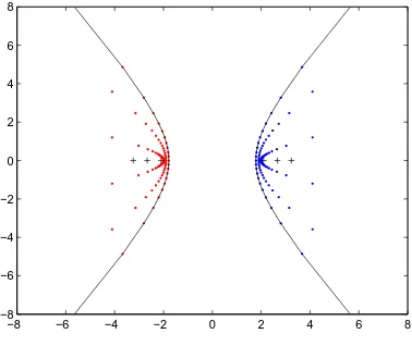
Example 3.2. Let A ∈ M6 be the tridiagonal matrix with a1 = 2, a2 = −2,
bj =iand cj =−2i,j = 1, . . . ,5.According to Theorem 2.2, WJ(A) is bounded by the hyperbola centered at (0,0) and with semi-transverse axis of length approximately 1.79.For σ+(HA) ={α1, α2, α3} and σ+(A) ={γ1, γ2, γ3}increasingly ordered and βj =γ2
j −α2j,j= 1, . . . ,6,the line equation of the boundary generating curve is
(w2−α21u2+β12v2)(w2−α22u2+β22v2)(w2−α23u2+β32v2) = 0.
The foci of the hyperbolas in Figure 3.1 are the eigenvalues ofA.
−8 −6 −4 −2 0 2 4 6 8
[image:12.612.163.352.250.409.2]−8 −6 −4 −2 0 2 4 6 8
Fig. 3.1.WJ(A)and boundary generating curves for the matrix of Example 3.2.
Observe that the boundary of theJ−numerical range of a tridiagonal matrix with biperiodic main diagonal may not be hyperbolic if the super and subdiagonals do not satisfy the conditions in Theorem 2.2.
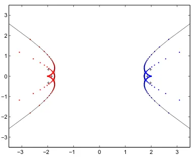
Example 3.3. LetJ =I1⊕ −I1⊕I1⊕ −I1⊕I1⊕ −I1 and letA∈M6be the
tridiagonal matrix with a1 = 2, a2 = −2, bj = 1, cj = −1 for j odd and cj = 1 for j even. There are two flat portions on the boundary, namely the line segments [√3 +i√6/6,√3−i√6/6] and [−√3 +i√6/6,−√3−i√6/6]. The line equation of the boundary generating curve is
−27u6+w2(v2+w2)2+ 3u4(8v2+ 9w2)−u2(4v4+ 14v2w2+ 9w4) = 0
and it is not factorizable (cf. Figure 3.2).
−3 −2 −1 0 1 2 3 −3
[image:13.612.162.351.111.272.2]−2 −1 0 1 2 3
Fig. 3.2.WJ(A)and boundary generating curves for the matrix of Example 3.3.
Example 3.4. Let
A=
4 0 −1 0 0 0
0 −4 0 −1 0 0
1 0 4 0 −1 0
0 1 0 −4 0 −1
0 0 1 0 4 + 2√2 0
0 0 0 1 0 −4 + 2√2
.
TheJ−numerical range ofA has one flat portion on the boundary, namely the line segment [4 +i,4−i] (cf. Figure 3.3).
4. Matlabprogram. In this section, we present the code for plotting the points defining the boundary generating curves of the J−numerical range of an arbitrary complex matrix. The program is listed below and is also available at the following website:
http://www.mat.uc.pt/∼bebiano
−8 −6 −4 −2 0 2 4 6 8 10 −4
[image:14.612.162.353.112.272.2]−3 −2 −1 0 1 2 3 4
Fig. 3.3.WJ(A)and boundary generating curves for the matrix of Example 3.4.
MATLAB PROGRAM FOR PLOTTING THE BOUNDARY GENERATING CURVE OF THEJ−NUMERICAL RANGE OF A COMPLEX MATRIX
%
%boundary_curve(A,J,m,Tol), where J is the J-Hermitian matrix that defines %the indefinite inner product, A is the Krein space matrix for which %the program computes points in the Krein space numerical range, 2m %is the number of directions and Tol>0 is the considered tolerance. %
function [X1_round,X2_round,degenerate1,degenerate2]=boundary_curve(A,J,m,Tol) %
global definite
X1_round=[]; X2_round=[]; %
if ~isequal(size(J,1),size(J,2)) error(’J must be a square matrix’); end
if ~isequal(size(A,1),size(A,2)) error(’A must be a square matrix’); end
if ~isequal(size(J),size(A))
error(’A and J must have the same size’); end
for r=1:size(J,2) for s=1:size(J,2)
end end end %
% Evaluation of the vector described in Step 1 [degenerate1,direc,eig_real]=directions(A,J,m,Tol); %
% Evaluation of the points of the boundary generating degenerate2=0;
if degenerate1~=1
row1=1; row2=1; X1=[]; X2=[]; vec=[]; for t=1:size(direc,2)
D1=[]; D2=[]; w=direc(t);
T=(exp(pi*i*(w-1)/(2*m))*A+ exp(-pi*i*(w-1)/(2*m))*J*A’*J)/2; [U,D]=eig(T);
for s=1:size(U,2) u=U(:,s);
if abs(real(u’*J*u))>=Tol %no null J-norm z2=real(u’*J*A*u)/real(u’*J*u); z3=imag(u’*J*A*u)/real(u’*J*u); if real(u’*J*u)>0 %positive J-norm
X1(row1)=z2+i*z3; row1=row1+1; D1=[D1 D(s,s)]; else
X2(row2)=z2+i*z3; row2=row2+1; D2=[D2 D(s,s)]; end
end end
for r=1:size(eig_real,2) if eig_real(r)==w
[interla]=interlacing(D1,D2); vec=[vec interla];
end end end %
%Cheking if there exists at least one direction %with noninterlacing eigenvalues
aux=0;
if vec(t)==2
aux=1; % Noninterlacing eigenvalues in the direction w=eig_real(t) break;
end end %
if aux==1 || definite==1
[X1_round]=rounding(X1); %Remove of rounding errors of X1 if definite==0
[X2_round]=rounding(X2); %Remove of rounding errors of X2 else
X2_round=[]; %Definite case end
%
%Plot of the boundary generating curves plot(real(X1_round),imag(X1_round),’.b’); hold on;
plot(real(X2_round),imag(X2_round),’.r’); hold on;
else
degenerate2=1; %Degenerate cases. return;
end end
Acknowledgment: The authors are very grateful to the referee for valuable sugges-tions.
REFERENCES
[1] N. Bebiano, R. Lemos, J. da Providˆencia, and G. Soares. On generalized numerical ranges of operators on an indefinite inner product space.Linear and Multilinear Algebra, 52:203–233, 2004.
[2] E. Brown and I. Spitkovsky. On matrices with elliptical numerical ranges.Linear and Multilinear Algebra, 52:177–193, 2004.
[3] M.-T. Chien. On the numerical range of tridiagonal operators. Linear Algebra and its Applica-tions, 246:203–214, 1996.
[4] M.-T. Chien. The envelope of the generalized numerical range. Linear and Multilinear Algebra, 43:363–376, 1998.
[5] M.-T. Chien and H. Nakazato. The c-numerical range of tridiagonal matrices. Linear Algebra and its Applications, 335:55–61, 2001.
[7] M. Fiedler. Numerical range of matrices and Levinger’s theorem. Linear Algebra and its Appli-cations, 220:171–180, 1995.
[8] M.J.C. Gover. The eigenproblem of a tridiagonal 2−Toeplitz matrix. Linear Algebra and its Applications, 197/198:63–78, 1994.
[9] C.-K. Li, N.K. Tsing, and F. Uhlig. Numerical ranges of an operator on an indefinite inner product space.Electronic Journal of Linear Algebra, 1:1–17, 1996.
[10] C.-K. Li and L. Rodman. Shapes and computer generation of numerical ranges of Krein space operators. Electronic Journal of Linear Algebra, 3:31–47, 1998.
[11] C.-K. Li and L. Rodman. Remarks on numerical ranges of operators in spaces with an indefinite inner metric. Proccedings of the American Mathematial Society, 126:973–982, 1998. [12] M. Marcus and B.N. Shure. The numerical range of certain 0,1-matrices.Linear and Multilinear
Algebra, 7:111–120, 1979.