LARGEST EIGENVALUES OF THE DISCRETE P-LAPLACIAN OF
TREES WITH DEGREE SEQUENCES∗
T ¨URKER BIYIKO ˘GLU†, MARC HELLMUTH‡, AND JOSEF LEYDOLD§
Abstract. Trees that have greatest maximum p-Laplacian eigenvalue among all trees with a given degree sequence are characterized. It is shown that such extremal trees can be obtained by breadth-first search where the vertex degrees are non-increasing. These trees are uniquely determined up to isomorphism. Moreover, their structure does not depend onp.
Key words. Discrete p-Laplacian, Largest eigenvalue, Eigenvector, Tree, Degree sequence, Majorization.
AMS subject classifications.05C35, 05C75, 05C05, 05C50.
1. Introduction. The eigenvalues of the combinatorial Laplacian have been intensively investigated during the last decades. Recently there is an increasing in-terest in the discrete p-Laplacian, a natural generalization of the Laplacian, which corresponds to p= 2; see e.g., [1–3, 9]. The related eigenvalue problems have been occasionally occurred in fields like network analysis [5, 10], pattern recognition [12], or image processing [6].
For a simple connected undirected graphG= (V, E) with vertex set V and edge setE thediscrete p-Laplacian ∆p(G) of a functionf onV (1< p <∞) is given by
∆p(G)f(v) =
u∈V,uv∈E
(f(v)−f(u))[p−1] .
We use the symbolt[q] to denote a “power” function that preserves the sign oft, i.e.,
t[q] = sign(t)· |t|q. Notice that for p = 2, ∆
2(G) is the well-known combinatorial
graph Laplacian, usually defined as ∆(G) = D(G)−A(G) where A(G) denotes the adjacency matrix ofG andD(G) the diagonal matrix of vertex degrees. For p= 2, ∆p(G) is a non-linear operator. We write ∆p (and ∆) for short if there is no risk of
confusion.
∗Received by the editors June 9, 2008. Accepted for publication March 17, 2009. Handling Editor:
Richard A. Brualdi.
†Department of Mathematics, I¸sık University, S¸ile 34980, Istanbul, Turkey
‡Department of Computer Science, Bioinformatics, University of Leipzig, Haertelstrasse 16–18,
D-04107 Leipzig, Germany ([email protected]).
§Department of Statistics and Mathematics, WU (Vienna University of Economics and Business),
A real numberλis called aneigenvalueof ∆p(G) if there exists a functionf = 0
onV such that
∆pf(v) =λ f(v)[p−1] .
(1.1)
The functionf is then called theeigenfunction corresponding toλ.
In this paper we are interested in the largest eigenvalue of ∆p(G), which we
denoted by µp(G). In particular we investigate the structure of trees which have
largest maximum eigenvalueµp(T) among all trees with a given degree sequence. We
call such treesextremal trees. We show that for such trees the degree sequence is non-increasing with respect to an ordering of the vertices that is obtained by breadth-first search. Furthermore, we show that the largest maximum eigenvalue in such classes of trees is strictly monotone with respect to some partial ordering of degree sequences. Thus, we extend a result that has been independently shown by Zhang [11] and Bıyıko˘glu et al. [4]. It is remarkable that this result is independent from the value of p. Although there is still little known about thep-Laplacian our result shows that it shares at least some of the properties with the combinatorial Laplacian.
2. Degree Sequences and Largest Eigenvalue. Letd(v) denote the degree of vertexv. We call a vertexv withd(v) = 1 a pendant vertex (orleaf) of a graph. Recall that a non-increasing sequence π= (d0, . . . , dn−1) of non-negative integers is
calleddegree sequence if there exists a graphGfor whichd0, . . . , dn−1are the degrees
of its vertices. In particular,πis a tree sequence, i.e. a degree sequence of some tree, if and only if every di >0 and ni=0−1di = 2 (n−1). We refer the reader to [7] for
relevant background on degree sequences. We denote the class of trees with a given degree sequenceπas
Tπ={Gis a tree with degree sequenceπ}.
We want to give a characterization of extremal trees inTπ, i.e., those trees inTπthat have greatest maximum eigenvalue. For this task we introduce an ordering of the vertices v0, . . . , vn−1 of a graph G by means of breadth-first search: Select a vertex
v0 ∈G and create a sorted list of vertices beginning with v0; append all neighbors
v1, . . . , vd(v0)ofv0 sorted by decreasing degrees; then append all neighbors ofv1that
are not already in this list; continue recursively with v2, v3, . . .until all vertices ofG
are processed. In this way we build layers where eachvin layeriis adjacent to some vertex w in layer i−1 and vertices uin layeri+ 1. We then call the vertexw the
parent ofvandv a child ofw.
Definition 2.1 (BFD-ordering). Let G = (V, E) be a connected graph with rootv0. Then a well-ordering≺of the vertices is calledbreadth-first search ordering
(B1) ifw1≺w2 thenv1≺v2for all childrenv1 ofw1andv2ofw2;
(B2) ifv≺u, thend(v)≥d(u).
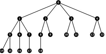
We call a connected graph that has a BFD-ordering of its vertices aBFD-graph (see Fig. 2.1 for an example).
0
1 2 3 4
5 6 7 8 9 10 11 12 13
[image:3.612.171.357.185.280.2]14 15 16 17 18
Fig. 2.1. A BFD-tree with degree sequenceπ= (42,34,23,110)
[image:3.612.196.321.366.438.2]Every graph has for each of its vertices v an ordering with root v that satisfies (B1). This can be found by a breadth-first search as described above. However, not all trees have an ordering that satisfies both (B1) and (B2); consider the tree in Fig. 2.2.
Fig. 2.2.A tree with degree sequenceπ= (42,21,16)where no BFD-ordering exists.
Theorem 2.2. A tree T with degree sequence π is extremal in class Tπ (i.e., has greatest maximum p-Laplacian eigenvalue) if and only if it is a BFD-tree. T is then uniquely determined up to isomorphism. The BFD-ordering is consistent with the corresponding eigenfunction f of G in such a way that |f(u)| > |f(v)| implies
u≺v.
For a tree with degree sequenceπa sharp upper bound on the largest eigenvalue can be found by computing the corresponding BFD-tree. Obviously finding this tree can be done inO(n) time if the degree sequence is sorted.
We now define a partial ordering on degree sequences π = (d0, . . . , dn−1) and
π′ = (d′
0, . . . , d′n′−1) with n≤n′ and π=π′ as follows: we writeπ⊳π′ if and only if j
i=0di ≤ j
i=0d′i for all j = 0, . . . , n−1 (recall that the degree sequences are
Theorem 2.3. Let πandπ′ be two distinct degree sequences of trees withπ⊳π′.
Let T and T′ be extremal trees in the classes Tπ andTπ′,respectively. Then we find
for the corresponding maximum eigenvalues µp(T)< µp(T′).
The following corollaries generalize results which are well-known for the case p= 2.
Corollary 2.4. A tree T is extremal in the class of all trees with nvertices if and only if it is the starK1,n−1.
Corollary 2.5. A treeGis extremal in the class of all trees withnvertices and
kleaves if and only if it is a star K1,kwith paths of almost the same lengths attached to each of itsk leaves. Almost means that each path of two leaves in the tree Ghas lengthl∈
2·n−1
k
,n−1
k
+n−1
k
,2·n−1
k
.
Proof. [of Cor. 2.4 and 2.5] The tree sequencesπn = (n−1,1, . . . ,1) andπn,k=
(k,2, . . . ,2,1, . . . ,1) are maximal w.r.t. ordering ⊳ in the respective classes of all
trees with nvertices and all trees withn vertices andk pendant vertices. Thus the statement immediately follows from Theorems 2.2 and 2.3.
3. Preliminaries. Thenon-linear Rayleigh quotient of ∆p(G) is given as [2, 9]
RpG(f) =
f,∆pf f, f[p−1] =
uv∈E|f(u)−f(v)| p
v∈V|f(v)|p
.
We can define a Banach space of real-valued functions on V using the p-norm of a function f, ||f||p = p
v∈V |f(v)|p, and a Banach space of a function F on the
directed edges [uv] using the norm |F|p = p
e∈E|F([uv])|p. Thus the Rayleigh
quotient can be written as [2]
RpG(f) = |∇f|p
p ||f||pp
,
where (∇f)([uv]) =f(u)−f(v) for an oriented edge [uv]∈E. Calculus of variation then implies the existence of eigenvalues and eigenfunctions. These are exactly the critical points of RpG(f) constrained to ||f||pp = 1 and can be found by means of
Lagrange multipliers (with then are the eigenvalues).
An immediate consequence of these considerations is that ∆p is a nonnegative
operator, i.e., the smallest eigenvalue is 0 and all other eigenvalues are strictly positive (in case of a connected graph). We find the following characterization of the largest eigenvalueµp(G) of ∆p(G) which generalizes the well-known Rayleigh-Ritz theorem.
Proposition 3.1 ([2]).
µp(G) = max ||f||p=1
RpG(f) = max ||f||p=1
uv∈E
Moreover,ifRpG(f) =µp(G)for a functionf,thenf is an eigenfunction correspond-ing to the maximum eigenvalueµp(G)of ∆p(G).
Notice that every eigenfunctionf corresponding to the maximum eigenvalue must fulfill the eigenvalue equation (1.1) for everyv∈V.
An eigenfunction f corresponding to the largest eigenvalueµp(G) has alternate
signs [2]. Thus the following observation simplifies our task. It generalizes a result of Merris [8]. Define thesignless p-Laplacian Qp(G) analog to the linear case by
Qp(G)f(v) =
u∈V,uv∈E
(f(v) +f(u))[p−1].
Its Rayleigh quotient is given by
QpG(f) = f, Qpf
f, f[p−1] =
uv∈E|f(u) +f(v)| p
v∈V |f(v)|p
.
Lemma 3.2. Let G= (V1∪˙V2, E) be a bipartite graph. Then ∆p(G)and Qp(G) have the same spectrum. Moreover, f is an eigenfunction of∆p(G) affording eigen-valueλif and only iff′is an eigenfunction ofQ
p(G)affordingλ,wherebyf′(v) =f(v) if v∈V1 andf′(v) =−f(v)if v∈V2.
Proof. Letf be an eigenfunction of ∆p(G), i.e., ∆pf(v) = u∈V,uv∈E(f(v)−
f(u))[p−1] = λf(v). Define s(v) = 1 if v ∈ V
1 and s(v) = −1 if v ∈ V2, hence
f′(v) = s(v)f(v). Then we find (Q
pf′)(v) = u∈V,uv∈E(f′(v) +f′(u))[ p−1] =
u∈V,uv∈Es(v)(f(v)−f(u))
[p−1] = λs(v)f(v)[p−1] = λf′(v)[p−1] and hence f′ is
an eigenfunction ofQp(G) affording the same eigenvalueλ, as claimed. The necessity
of the condition follows analogously.
Hence we will investigate the eigenfunction to the maximum eigenvalue ofQp(G)
in our proof. Prop. 3.1 holds completely analogously for the maximum eigenvalue.
Proposition 3.3.
µp(G) = max ||f||p=1
QpG(f) = max
||f||p=1
uv∈E
|f(u) +f(v)|p
.
Moreover,ifQpG(f) =µp(G)for a functionf,thenf is an eigenfunction correspond-ing to the maximum eigenvalueµp(G)of Qp(G).
We call a positive eigenfunction f corresponding to µp(G) a Perron vector of
Q(G). The following technical result will be useful.
Lemma 3.5. Let 0 ≤ ǫ ≤ δ ≤ z and p > 1. Then (z+ǫ)p + (z −ǫ)p ≤
(z+δ)p+ (z−δ)p. Equality holds if and only ifǫ=δ.
Proof. Obviously equality holds when ǫ = δ. Let ǫ < δ. Notice that tp is
strictly monotonically increasing and strictly convex for every t ≥0. Thus we find (z−ǫ)p−(z−δ)p<(δ−ǫ)p(z−ǫ)p−1and (z+ǫ)p−(z+δ)p<−(δ−ǫ)p(z+ǫ)p−1
by using tangents inz−ǫandz+ǫ, respectively. Consequently (z−ǫ)p−(z−δ)p+
(z+ǫ)p−(z+δ)p < p(δ−ǫ) ((z−ǫ)p−1−(z+ǫ)p−1)≤0 and thus the statement
follows.
4. Proof of the Theorems. Because of Lemma 3.2 we characterize trees that maximize the largest eigenvalue µp(G) of Qp. In the following f always denotes a
Perron vector ofQp(T) for some tree T. Puv denotes the path between two vertices
uandv.
The main techniques for proving our theorems isrearranging of edges. We need two types of rearrangement steps that we callswitching andshifting, respectively, in the following.
Lemma 4.1 (Switching). Let T ∈ Tπ and let u1v1, u2v2 ∈E(T)be edges such
that the pathPv1v2 neither containsu1 noru2,andv1=v2. Then by replacing edges
u1v1 and u2v2 by the respective edges u1v2 and u2v1 we get a new tree T′ ∈ Tπ.
Furthermore, µ(T′) ≥ µ(T) whenever there exists a Perron vector f with f(u
1) ≥
f(u2)andf(v2)≥f(v1),andµ(T′)> µ(T)if one of the two inequalities is strict.
Proof. SincePv1v2 neither containsu1 noru2 by assumption, T′ is again a tree.
Since switching of two edges does not change degrees,T′also belongs to classTπ. Let f be a Perron vector with||f||p= 1. To verify the inequality we have to compute the effects of removing and inserting edges on the Rayleigh quotient.
µp(T′)−µp(T)≥ QpT′(f)− Q
p T(f)
= [ (f(u1) +f(v2))p+ (f(v1) +f(u2))p]
−[(f(v1) +f(u1))p+ (f(u2) +f(v2))p]
˙
=D1p+D2p−D3p−D4p
≥0.
The last inequality follows from Lemma 3.5 by setting z+δ = D1, z−δ = D2,
z+ǫ = max{D3, D4}, and z−ǫ = min{D3, D4}. Notice that D1 +D2 = D3+
D4 and that D1 ≥ D3, D4 ≥ D2. If f(u1) > f(u2) or f(v2) > f(v1) then the
eigenvalue equation (1.1) would not hold forv1oru2. Thusf is not an eigenfunction
Lemma 4.2 (Shifting). Let T ∈ Tπ and u, v ∈ V(T) with u = v. Assume we have edges ux1, . . . , uxk ∈E(T) such that none of the xi is in Puv. Then we get a new graph T′ by replacing all edgesux
1, . . . , uxk by the respective edgesvx1, . . . , vxk. Moreover,µp(T′)> µp(T)whenever there exists a Perron vectorf withf(u)≤f(v).
Proof. Letf be a Perron vector with||f||p= 1. Then
µp(T′)−µp(T)≥ QpT′(f)− QpT(f)
=k
i=1[(f(v) +f(xi))p−(f(u) +f(xi))p] ≥0.
where the last inequality immediately follows from the strict monotonicity of tp for
everyt ≥0. Now ifµp(T′) =µp(T) then f also must be an eigenfunction of T′ by
Lemma 3.3. Thus the eigenvalue equation (1.1) for vertexuinT andT′ implies that f(u) +f(xi) = 0, a contradiction, sincef is strictly positive on each vertex.
Lemma 4.3. Let T be extremal in class Tπ andf a Perron vector of Qp(T). If
d(u)> d(v),thenf(u)> f(v).
Proof. Suppose d(u)> d(v) but f(u)≤f(v). Then we construct a new graph T′∈ Tπ by shiftingk=d(u)−d(v) edges in T. For this task we can choose anyk of
thed(u)−1 edges that are not contained inPuv. Thusµp(T′)> µp(T) by Lemma 4.2,
a contradiction to our assumption thatT is extremal.
Lemma 4.4. Each class Tπ contains a BFD-treeT that is uniquely determined up to isomorphism.
Proof. For a given tree sequence the construction of a BFD-tree is straightforward. To show that two BFD-trees T andT′ in classTπ are isomorphic we use a function
φthat maps the vertexvi in theith position in the BFD-ordering ofT to the vertex
wi in theith position in the BFD-ordering ofT′. By the properties (B1) and (B2)φ
is an isomorphism, asvi andwi have the same degree and the images of neighbors of
vi in the next layer are exactly the neighbors ofwi in the next layer.
Now letT be an extremal tree inTπwith Perron vectorf. Create an ordering≺
of its vertices by breadth-first search starting with the maximum off. For all children ui of a vertexwwe set ui≺uj whenever
(i) f(ui)> f(uj) or
(ii) f(ui) =f(uj) andd(ui)> d(uj).
We enumerate the vertices ofT with respect to this ordering, i.e.,vi ≺vj if and only
ifi < j. In particular,v0is a maximum of f.
Proof. Suppose we have two verticesvi≻vj withf(vi)> f(vj). Letwk be the
first vertex (in the ordering≺) which has such a childvjwith this property, and choose
vi (≻ vj) as the first vertex with f(vi) > f(vj). Since v0 is a maximum off such
a wk must exist. By construction of our breadth-first search we havewk ≺vj ≺vi,
wkvi∈E(T), andf(wk)≥f(u) for allu≻wk. We have two cases:
(1) vjis in the pathPwkvi: Thenf(vi)> f(vj) and Lemma 4.3 implyd(vi)≥d(vj)≥ 2 and thus there exists a childwmofvi which cannot be adjacent tovj.
(2) vj is not in the path Pwkvi: Then the parentwmof vi cannot be adjacent tovj. Moreover,wm≻wk since otherwise vi≺vj.
In either case we find f(wk) ≥ f(wm) and f(vi) > f(vj). Thus we can replace
edges wkvj and wmvi by the edgeswkvi and wmvj we get a new treeT′ ∈ Tπ with
µp(T′)> µp(T) by Lemma 4.1, a contradiction to our assumption.
Proof of Theorem 2.2. Again use the above ordering ≺. Thus (B1) holds. By Lemma 4.5f is monotone with respect to this ordering. Thus Lemma 4.3 (together with construction rule (ii)) implies (B2). The sufficiency of our condition is a conse-quence of the uniqueness of BFD-trees as stated in Lemma 4.4.
Proof of Theorem 2.3. Letπ={d0, . . . , dn−1} and π′ ={d′0, . . . , d′n′−1} be two tree sequences with π⊳π′ andn=n′. By Theorem 2.2 the maximum eigenvalue is
largest for a treeT within classTπ whenT is a BFD-tree. Againf denotes a Perron vector ofQp(T). We have to show that there exists a treeT′∈ Tπ′ such thatµ(T′)> µ(T). Therefore we construct a sequence of treesT =T0 →T1→. . .→Ts=T′ by
shifting edges and show that µp(Tj) > µp(Tj−1) for every j = 1, . . . , s. We denote
the degree sequence ofTj byπ(j).
For a particular step in our construction, let k be the least index with d′k >
d(kj). Let vk be the corresponding vertex in treeTj. Since ki=0d′i >
k
i=0d (j)
i and
n−1
i=0 d′i =
n−1
i=0 d (j)
i = 2(n−1) there must exist a vertex vl ≻ vk with degree
d(lj)≥2. Thus it has a childul. By Lemma 4.2 we can replace edgevlulby edgevkul
and get a new tree Tj+1 with µp(Tj+1)> µp(Tj). Moreover, d( j+1)
k =d
(j)
k + 1 and
d(lj+1)=d(lj)−1, and consequentlyπ(j)⊳π(j+1). By repeating this procedure we end
up with degree sequenceπ′ and the statement follows for the case wheren′=n.
Now assume n′ > n. Then we construct a sequence of trees Tj by the same
procedure. However, now it happens that we arrive at some treeTr whered′k > d
(r)
k
but d(lr) = 1 for all vl ≻ vk, i.e., they are pendant vertices. In this case we join a
new pendant vertex tovk. Then d
(r+1)
k =d
(r)
k + 1 and we have added a new vertex
degree of value 1 to π(r) to obtainπ(r+1). Thusπ(r+1) is again a tree sequence with
π(r)⊳π(r+1). Moreover,µ
p(Tr+1)> µp(Tr) asTr+1⊃Tr. By repeating this procedure
References.
[1] S. Amghibech. Eigenvalues of the discretep-Laplacian for graphs. Ars Comb., 67:283–302, 2003.
[2] S. Amghibech. Bounds for the largestp-Laplacian eigenvalue for graphs.Discrete Math., 306:2762–2771, 2006. doi: 10.1016/j.disc.2006.05.012.
[3] S. Amghibech. On the discrete version of Picone’s identity.Discrete Appl. Math., 156:1–10, 2008. doi: 10.1016/j.dam.2007.05.013.
[4] T¨urker Bıyıko˘glu, Marc Hellmuth, and Josef Leydold. Largest Laplacian eigen-value and degree sequences of trees, 2008. URLarXiv:0804.2776v1 [math.CO]. [5] Takashi Kayano and Maretsugu Yamasaki. Boundary limit of discrete Dirichlet
potentials. Hiroshima Math. J., 14(2):401–406, 1984.
[6] Olivier Lezoray, Abderrahim Elmoataz, and S´ebastien Bougleux. Graph regular-ization for color image processing. Computer Vision and Image Understanding, 107(1–2):38–55, 2007.
[7] O. Melnikov, R. I. Tyshkevich, V. A. Yemelichev, and V. I. Sarvanov. Lectures on Graph Theory. B.I. Wissenschaftsverlag, Mannheim, 1994. Translation from Russian by N. Korneenko with the collaboration of the authors.
[8] Russel Merris. Laplacian matrices of graphs: A survey. Linear Algebra Appl., 197–198:143–176, 1994.
[9] Hiroshi Takeuchi. The spectrum of thep-Laplacian andp-harmonic morphisms on graphs. Illinois J. Math., 47(3):939–955, 2003.
[10] Maretsugu Yamasaki. Ideal boundary limit of discrete Dirichlet functions. Hi-roshima Math. J., 16(2):353–360, 1986.
[11] Xiao-Dong Zhang. The Laplacian spectral radii of trees with degree sequences.
Discrete Math., 308(15):3143–3150, 2008.