The Role of Abilities and Schooling Choices
Sergio Urzu´a
a b s t r a c t
This paper studies the relationship between abilities, schooling choices, and black-white differentials in labor market outcomes. The analysis is based on a model of endogenous schooling choices. Agents’ schooling decisions are based on expected future earnings, family background, and unobserved abilities. Earnings are also determined by unobserved abilities. The analysis distinguishes unobserved abilities from observed test scores. The model is implemented using data from the NLSY79. The results indicate that, even after controlling for abilities, there exist significant racial labor market gaps. They also suggest that the standard practice of equating observed test scores may overcompensate for differentials in ability.
I. Introduction
The existence of black-white gaps in a variety of labor market and educational outcomes has been extensively documented. It is well established that, on average, blacks are less educated, have lower income, and accumulate less work experience than whites.1This paper studies whether the differences in labor market outcomes and schooling attainment can be interpreted as the manifestation of black-white ability differentials. Although this idea is not new, the analysis presented is a
Sergio Urzu´a is a professor of economics at Northwestern University, Department of Economics, 2001 Sheridan Road, Office 302, Evanston IL 60208; telephone: 847-491-8213; email:
s-urzua@northwestern.edu. The author is indebted to James Heckman for his encouragement and guidance throughout this project. He acknowledges helpful discussions with Derek Neal, Glenn Loury, Robert Townsend, Lars Hansen, Chris Taber, Greg Duncan, Jora Stixrud, Paul LaFontaine, three anonymous referees, and the participants in workshops at the University of Chicago, Brown University, Northwestern University, the 2007 ASSA/AEA Meeting, and at the Third Chicago Workshop on Black-White Inequality. The usual disclaimer applies. Supplementary material: http://
faculty.wcas.northwestern.edu/;ssu455/research/gapWebAppendix.pdf. The data used in this article can be obtained beginning May 2009 through April 2012 from Sergio Urzu´a, Northwestern University, Department of Economics, 2001 Sheridan Road, Office 302, Evanston IL 60208; telephone: 847-491-8213; email: s-urzua@northwestern.edu
½Submitted May 2006; accepted June 2007
ISSN 022-166X E-ISSN 1548-8004Ó2008 by the Board of Regents of the University of Wisconsin System
T H E J O U R NA L O F H U M A N R E S O U R C E S d X L I I I d 4
comprehensive one that takes into account several aspects that have been only par-tially recognized in the literature.
The empirical strategy utilized in this paper treats both schooling decisions and labor market outcomes as endogenous variables. This represents an important differ-ence relative to previous studies, as schooling decisions are usually either excluded from the analysis on the grounds that they might be influenced by discrimination (Neal and Johnson 1996), or included under the presumption that they can be treated as exogenous variables (Lang and Manove 2006).2The omission of schooling obvi-ously prevents the study of black-white differences in educational decisions and the extent to which those differences explain the observed gaps in labor market out-comes. Their inclusion as exogenous variables, on the other hand, limits the scope of the empirical analysis because of potential endogeneity bias.
Also addressed is the extent to which black-white gaps can be explained by non-cognitive, as well as non-cognitive, ability differentials. This is particularly relevant since recent studies have demonstrated that noncognitive abilities are as important as, if not more important than, cognitive abilities in determining labor market, educational, and behavioral outcomes (for example, Bowles, Gintis, and Osborne 2001a,b; Farkas 2003; and Heckman, Stixrud, and Urzua 2006). However, to date very little is known about the role these abilities play in explaining racial differentials.
Importantly, the analysis distinguishes observed cognitive and noncognitive meas-uresfrom unobserved cognitive and noncognitiveabilities. This distinction is based on the idea that observed (or measured) abilities are the outcome of a process involving familial inputs, schooling experience, and pure (unobserved) ability. The relevance of this distinction comes from the claim that racial gaps in observed achievement tests (interpreted as observed cognitive abilities or premarket factors) can explain most of the racial differences in labor market outcomes (see, for example, Neal and Johnson 1996). If racial differences in achievement test scores do not emerge exclusively as the result of differences in abilities but also as the result of differences in family background and schooling environment, then by comparing the labor mar-ket outcomes of blacks and whites with similar observed abilities (test scores), we are not necessarily understanding or identifying the real factors behind the racial gaps. The analysis of this paper sheds light on this point.3
Finally, although the analysis mainly focuses on black-white differences in labor market outcomes and schooling decisions, it also addresses whether ability
2. An important exception is the analysis of Keane and Wolpin (2000). Keane and Wolpin (2000) analyze racial labor market gaps using a dynamic model of schooling, work, and occupational choice decisions with unobserved heterogeneity (endowments). However, unlike the analysis in this paper, they do not link the unobserved endowments to specific abilities.
differentials can explain racial differences in incarceration. The racial differences in this dimension of social behavior have received increasing attention in the literature.4 The empirical results of the paper establish the existence of racial differences in the distributions of cognitive and noncognitive abilities. They also demonstrate that, regardless of the racial group analyzed, these abilities are important determinants of labor market outcomes and schooling attainment, and document the existence of sig-nificant differences across racial groups in the way these abilities determine each of these dimensions. This is particularly clear in the case of schooling attainment, where noncognitive abilities have stronger positive effects among blacks than among whites. The results also confirm that racial gaps in labor market outcomes reduce after con-trolling for cognitive abilities. However, the percentage explained by these abilities is significantly smaller than what has been previously claimed in the literature. This is a direct consequence of the distinction between observed and unobserved abilities. More-over, although there are significant black-white differences in noncognitive abilities, they play a minor role in explaining gaps in labor market outcomes. However, noncognitive abilities help to explain a significant fraction of the racial gaps in incarceration rates.
It is important to notice that it is not an objective of this paper to provide a comprehen-sive explanation of the factors explaining the racial differences in unobserved abilities. Specifically, in the context of the empirical model described in this paper, and given the data limitations,5the estimated racial differences in unobserved abilities could be the result of a variety of unobserved factors (unmeasured racial differences in early family environment including prenatal family environment, unmeasured racial differences in early schooling environment, cultural differences between groups, biological/genetic dif-ferences between groups, or, most likely, a combination of all of these). There is nothing in this paper that contradicts this argument, and consequently, the existence (and explan-atory power) of the ability differentials must be interpreted in this context.
The paper is organized as follows. Section II presents evidence on the black-white wage gap using the standard empirical approach. The results from Section II motivate the main ideas of the paper. Section III introduces the model of endogenous labor mar-ket outcomes, schooling decisions, and unobserved abilities, while Section IV analyzes the relationship between test scores and abilities in the context of the model. This sec-tion also introduces the model for incarcerasec-tion. Secsec-tion V discusses the empirical implementation of the model. Section VI presents the main results and examines whether black-white gaps in labor market outcomes, schooling choices, and incarcera-tion rates can be explained by racial differences in abilities. Secincarcera-tion VII concludes.
II. Background and Motivation
This section motivates the main ideas of the paper by utilizing a con-ventional reduced-form approach to analyze black-white differentials in labor market outcomes. Specifically, consider the following linear model for a labor market out-comeY(usually hourly wages or earnings):
4. Freeman (1991), Bound and Freeman (1992), Grogger (1998), Western and Pettit (2000).
lnY¼uBlack+gTest+ +S s¼1
fsDs+U ð1Þ
whereBlackrepresents the race dummy,Dsrepresents a dummy variable that takes a value of one if the individual’s schooling level iss (withs¼1,..,S),Testrepresents an ability measure (observed ability),6andUis the error term in the regression. Different versions of Equation 1 can be found in the literature studying black-white inequality in the labor market.7Here, the coefficient associated with the race dummy can be written as
u¼E½lnYjBlack¼1;Test;Ds2E½lnYjBlack¼0;Test;Ds ð2Þ
for any schooling levels, soucan be interpreted as the mean racial difference in (log) labor market outcomeYafter controlling for measured ability and schooling decisions. In other words,urepresents the difference between two individuals that share the same levels of education and measured ability, and differ only in their races.
Although the logic behind Equation 1 is simple and intuitive, its empirical imple-mentation requires some non-trivial considerations. The first concern is the existence of unobserved variables simultaneously affecting schooling decisions and labor mar-ket outcomes. The consequences of this potential endogeneity on the estimates of the returns to schooling (eachfsin Equation 1) have received the attention of many for more than 50 years (Mincer 1958 and Becker 1964). The instrumental variable ap-proach has emerged as the most popular method to deal with this endogeneity prob-lem (Card 2001). However, less attention has been paid to the consequences of endogeneity bias in the estimates ofu.
Neal and Johnson (1996) propose a different empirical strategy that, in principle, avoids concerns about endogeneity biases. They addressed a specific counterfactual. Namely, if two young people with the same basic reading and math skills reach the age at which schooling is no longer mandatory, how different will their labor market outcomes be when they are prime working age adults? Neal and Johnson (1996) were not interested in how choices made concerning education, labor supply, or occupa-tion might shape the wage and earnings profiles of blacks and whites differently. Rather, they focused only on the average differences in outcomes among persons who began making adult choices concerning education and labor supply given the same endowments of basic skills (proxied by achievement test scores).8
6. In general,Testcould represent a vector containing both observed cognitive and noncognitive abilities. 7. See Neal (2008), Farkas et al. (1997), Altonji and Blank (1999), and Farkas (2003).
8. Neal and Johnson (1996) exclude the schooling dummies from Equation 1 on the grounds that they can be influenced by discrimination. In this way, the endogenous variables are absorbed into the error term of the regression. However, the exclusion of schooling opens the door to a new source of potential problems in the estimation ofu, due to the omission of relevant variables. But, under the logic of Neal and Johnson (1996), this does not represent a problem. Because the biased OLS estimator ofuðuOLSÞwould contain,
in this case, the indirect effect of race on the schooling dummies (controlling for the observed ability), uOLScould still be interpreted as an estimate of the overall mean racial difference in the outcome (log)
Yeven if the schooling dummies are excluded. Specifically, in the Neal and Johnson’s specification, the OLS estimate of the coefficient associated with the race dummy would identify the following object: u++fs½PrðDs¼1jBlack¼1;TestÞ2PrðDs¼1jBlack¼0;TestÞ, where the second term represents
By contrast,uin Equation 2 defines a different racial gap in labor market outcomes that has been the focus of a large literature. If two young persons of different races begin their adult lives with similar ability levels and then make comparable investment in their human capital, how much will their wages differ as adults? As the analysis of this paper will show, a fixed racial gap in wages will not provide a satisfactory answer to this question. Among black and white persons who begin their adult lives with comparable abilities, racial differences in adult wages and earnings will vary among groups that choose different levels of educational investment. The empirical approach utilized in this paper will allow me to estimate these different racial gaps and also make progress toward understanding why changes in investment behavior among blacks have not equalized black and white returns to different levels of schooling.
A second concern when implementing Equation 1 is whether observed ability (Test) measures ability accurately. Several studies have demonstrated that observed ability measures cannot be interpreted as pure abilities and that they are influenced by home and school environments (see Neal and Johnson 1996; Todd and Wolpin 2003; and Cunha et al. 2006 for evidence). This simple consideration has important consequences for the interpretation of the OLS estimates ofu. In fact, if pure ability were the determinant of the outcomeY, and if, in the estimation of Equation 1, a proxy for ability (Test) were used instead, the OLS estimator of the racial gapuwould be biased in an unpredictable way. An additional concern regarding the estimation of Equation 1, which has a direct implication for the way the gap is defined (Equation 2), comes from the assumptions on the parameters of the model. A specification like Equation 1 assumes that black and white subjects face the same returns to observed ability and schooling, that is, the same g,f1,.,fS.The convenience of this assumption is clear: if the returns are the same, the black-white gap can be measured directly by a singleu. However, the assumption of equal returns can—and should—be tested. The assumption of a singleurepresents a simplification imposed a priori in Equation 1.
A natural extension of Equation 1 would be a specification in whichuis allowed to vary across schooling levels. However, the implementation of such a model also would require taking into account the fact that individuals may decide the schooling levels based on the potential differences in these returns. Therefore, this approach would naturally generate concerns about the endogeneity of schooling decisions.9
The main objective of this paper is the estimation of the black-white gaps in labor market outcomes using an approach that takes into account each of these issues. That is, the empirical model used in this paper deals with the endogeneity of schooling choices, the measurement error problem in abilities (cognitive and noncognitive abil-ities), and the unnecessary restrictions that are usually imposed a priori in the empir-ical literature. But, before introducing the model and its results, it is informative to follow the standard approach and to present the estimated black-white gaps in labor market outcomes (wages and earnings) as computed using OLS on some of the tra-ditional specifications of Equation 1 found in the literature. These results will serve as a comparison later in the paper.
Table 1 presents the black-white gaps in log hourly wages and log annual earnings obtained from four different specifications of Equation 1. The gaps are estimated using a representative sample of males from the National Longitudinal Survey of Youth 1979 (NLSY79).10The specifications differ exclusively in the set of controls included in the equations.
The first specification (Model A in Table 1) presents the baseline model. It includes only variables associated with an individual’s place of residence as con-trols.11 The estimated black-white gaps in log hourly wages and log earnings are 0.294 and 0.567, respectively. Using the traditional interpretation of these results, it is possible to conclude that, on average, blacks make approximately 25 percent less per hour and 43 percent less per year than whites.12Both numbers are substantial in magnitude and similar to what has been found in the literature (Neal and Johnson 1996; Neal 2008). They are also statistically significant (as are all of the numbers presented in the table). When schooling dummies are included as controls (Model B), the gaps reduce to 0.230 and 0.482 for hourly wages and annual earnings, respec-tively.13These numbers imply a significant reduction in the gaps when compared with the estimates from the baseline model (Model A).
However, the estimated gaps should not be compared across models, as each model represents a different specification. Specifically, in order to correctly quantify the reduction in the gap due to schooling, we must compare the estimated gap from Model B with the mean black-white difference in outcome after expecting out the effects of the schooling dummies from Model B. More precisely, in the context of the two models
lnY¼uABlack+UA ðModel AÞ
lnY¼uBBlack+ +S s¼1
fsDs+UB ðModel BÞ; ð3Þ
we must compareuB
versusuB++S
s¼1fsðE½DsjBlack¼12E½DsjBlack¼0Þ, in-stead of uB versus
uA. Under Model B in Table 1, Row 1 presents
uB whereas Row 2 presents the gap after expecting out the schooling dummies, that is, uB++S
s¼1fs ðE½DsjBlack¼12E½DsjBlack¼0Þ. By comparing these numbers,
10. The NLSY79 is widely used for the analysis of black-white gaps in wages, earnings, and employment. It contains panel data on wages, schooling, and employment for a cohort of young persons, aged 14 to 22 at their first interview in 1979. This cohort has been followed ever since. See Data Appendix 2 for details of the sample used in this paper.
11. Specifically, Model A includes as controls the dummy variables: northcentral region, northeast region, south region, west region and urban area.
12. The 25 percent is calculated as 1-exp(-0.29). Likewise, 43 percent is calculated as 1-exp(-0.567). No-tice that these calculations omit the fact thatE½lnYis not the same as lnE½Y.
Black-White Gaps Baseline Baseline Baseline Baseline
+ + +
Schooling Cognitive Schooling Dummies Test Score Dummies
+ Cognitive Test Score
(A) (B) (C) (D)
Wages Earnings Wages Earnings wages Earnings wages Earnings
(1) Black-White Gap 20.294 20.567 20.230 20.482 20.099 20.287 20.125 20.326
Black-White Gap Conditional on:
(2) Baseline Variables 20.294 20.567 20.292 20.572 20.302 20.578 20.299 20.579 (3) Baseline Variables Schooling Dummies 20.230 20.482 — — 20.265 20.532 (4) Baseline Variables and Cognitive Test Score 20.099 20.287 20.159 20.373 (5) Baseline Variables, Schooling Dummies, and
Cognitive Test Score
20.125 20.326
Notes: Model (A) (baseline model): log wages or log earnings are regressed on a race dummy (Black¼1) and a set of variables controlling for the characteristics of the place of residence (northcentral region, northeast region, west region and urban area). Models (B) and (D): The regressions include a set of dummy variables controlling for schooling levels (high school dropouts, high school graduates, some college, and four year college graduates). The schooling levels correspond to the maximum schooling level observed for each individual in the sample. Models (C) and (D): The regressions include the standardized average of six achievement test scores (Arithmetic Rea-soning, Word Knowledge, Paragraph Comprehension, Numerical Operations, Math Knowledge, Coding Speed). Wages and earnings represent the average value reported between ages 28 and 32.
Finally, for each model, Row 1 in Table 1 presents the gaps defined conditional on all the controls included in the regression. Rows 2-5 present the gaps defined condi-tioning on subsets of controls. For example, in the case of Model (D), where the respective labor market outcome lnY(hourly wages or annual earnings) is regressed on the baseline variables (X), schooling dummiesðfDsgSs¼1Þ, and the proxy for cognitive ability (Test) (the standardized average of achievement test scores), Table 1 presents EðlnYBlack
2lnYWhitejXÞ(Row 2),EðlnYBlack
2lnYWhitejX;fD
sgSs¼1Þ(Row 3),EðlnYBlack2lnYWhitejX;TestÞ(Row 4), andEðlnYBlack2lnYWhitejX;fDsgSs¼1;TestÞ(Row 5). It is worth noting that, in the case of Model (D), the estimates in Row 5 are identical to the ones in Row 1 since in both cases they represent the coefficient associated with the race dummy orEðlnYBlack
2lnYWhitejX;fD
sgSs¼1;TestÞ. That is why the numbers in Row 5 are presented in bold. The same logic applies to the other columns. Thus, each row in Table 1 presents black-white gaps that are comparable across columns (models), and for each column the bold number represents the gap estimated as the coefficient associated with the race dummy. All of the estimates are statistically significant at the five percent level.
Urzu
´a
we can conclude that schooling seems to reduce the coefficient associated with the race dummy (the gap) by 21 percent or 16 percent, depending on the labor market outcome considered.
Model C in Table 1 presents the results from the specification proposed by Neal and Johnson (1996). Thus, in addition to the baseline variables, the model includes a proxy for an individual’s cognitive ability or intelligence. This proxy is a stan-dardized average computed using six achievement tests available in the NLSY79 sample.14The estimated gaps are, in this case, 0.099 and 0.287 for wages and earn-ings, respectively. These numbers represent reductions in the estimated gaps for (log) wages and (log) earnings of 67 percent and 50 percent (Row 1 versus Row 4 under Model C), respectively, which are in the range of what has been found in the literature (see Carneiro, Heckman, and Masterov 2005; Neal and Johnson 1996).
The evidence from Models B and C suggests that both schooling and cognitive ability help to reduce the black-white gaps in wages and earnings. Model D studies the effects on the gap when they are simultaneously included in the regressions. The results in this case indicate that, when schooling and cognitive ability are con-trolled for, the estimated black-white gaps are 0.125 (wages) and 0.326 (earnings) (see Row 1 under Model D), with associated gap reductions of 58 percent and 44 percent (Row 1 versus Row 5 under Model D), respectively. Notice that these reductions are smaller in magnitude than the ones obtained when schooling varia-bles are omitted from the analysis (Model C), and so the results seem to indicate that schooling has unequal effects on labor market outcomes.15 However, this would (again) be the wrong comparison. A closer look at the evidence from Model D suggests that when the contribution of schooling is measured correctly (Row 3 versus Row 2), it implies a reduction of 11 percent in the wage gap (0.265 versus 0.299) and 8 percent in the earnings gap (0.532 versus 0.579). Thus, schooling var-iables seem to explain sizeable proportions of the gaps. Likewise, when only the contribution of cognitive ability is analyzed (Row 4 versus Row 2), I obtain reduc-tions of 47 percent in the wage gap (0.159 versus 0.299) and 36 percent in the earn-ings gap (0.373 versus 0.579). Overall, the evidence from Model D suggests that cognitive ability reduces the gap the most, although the contribution of cognitive ability is less than the one obtained from Model C.
In summary, the results in Table 1 suggest that the proxy for cognitive ability (av-erage achievement test score) is the most important explanatory variable of the black-white gaps in wages and earnings. This is consistent with previous findings in the literature. Its explanatory power is maximized when it is the only variable in-cluded in the model (other than the baseline variables), and it decreases when
schooling is included as a control. Schooling on the other hand, explains an impor-tant fraction of the gaps in wages and earnings.16
However, as previously explained, these results are subject to important qualifica-tions. Firstly, it is not completely clear what the proxy for cognitive ability is really measuring. Achievement test scores are known to not only be the results of pure abil-ity, but also of home and school environments (see Neal and Johnson 1996; Todd and Wolpin 2003; and Cunha et al. 2006). Additionally, the results do not consider the potential role of noncognitive abilities (such as self-motivation, self-esteem, and self-control, among others) as explanatory factors of the black-white inequality. Fur-thermore, by estimating an overall gap and treating schooling as an exogenous vari-able, these results do not provide a deep and precise understanding of the extent to which blacks and whites differ in terms of labor market outcomes. An integrated ap-proach in which schooling choices are modeled jointly with wages is needed. This approach is discussed below.
III. The Model of Labor Market Outcomes and
Schooling Choices
This section presents a model that integrates labor market outcomes (hourly wages, annual hours worked, and annual earnings) with schooling choices for the analysis of racial labor market gaps. The model assumes that individuals make their schooling choices based on their expectation about future labor market out-comes and schooling costs.
For sake of notational simplicity, I omit the supra-index for race in the exposition of the model, but the reader should be aware that every parameter in the model is defined separately for blacks and whites; that is, that the model applies separately to each race.
A. The Schooling Decision
The model considersT+1 time periods (t¼0,1,.,T) andSpossible schooling levels (s¼1,.,S). Each individual chooses his final schooling level att¼0 and receives la-bor income at the end of each period (except period 0). The stream of lala-bor income depends on the schooling level selected.
Individuals make their schooling decisions based on a comparison of the expected benefits and costs associated with each alternative. Specifically, if Vs denotes the expected benefit associated with schooling levels, then
Vs¼E + T
t¼1
rt+ 1uðEsðtÞÞj I0
;
whereu() represents the per period utility function,Es(t) represents the total earnings received in periodtgiven schooling levels,ris the discount factor, andI0represents the information set available to the agent att¼0. The information contained inI0is discussed below.
Total earnings received at the end of periodt are simply the product of hourly wages (Ys(t)) and total number of hours worked during the period (Hs(t)), that is, EsðtÞ ¼YsðtÞ3HsðtÞ. Notice that both wages and hours depend on the schooling level and time period.
Additionally, each schooling level has attached a schooling costGs. This cost can include not only monetary expenses associated with the specific schooling level (tu-ition, for example), but also associated psychic costs.17Gsmust bepaidby the indi-vidual at the time the decision is made. Thus, the net expected value (V˜s) associated with schooling levels is
V ;
s¼E +
T
t¼1
rt+ 1uðYsðtÞ3HsðtÞÞ2Gsj I0
fors¼1;.;S: ð4Þ
The individual selects his schooling level s* at period t¼0 by comparing the expected net utility levelsV˜sacross the differentSalternatives.
B. Labor Market Outcomes and Schooling Costs
The models for (log) hourly wages (Ys(t)) and (log) hours worked (Hs(t)) are
YsðtÞ ¼uYs;t+bYs;tXt+UYs;t ð5Þ
HsðtÞ ¼uHs;t+bHs;tQt+UHs;tfors¼1;.;Sandt¼1;.;T; ð6Þ
whereXtandQtrepresent the exogenous vectors of variables determining the labor outcomes, andUYs;tandUHs;trepresent the associated unobserved components in the equations. Equations 5 and 6 show how the individual’s labor market outcomes de-pend on the specific schooling level and time period considered.
Schooling costs associated with schooling levels are modeled as
Gs¼uGs+gsPs+esfors¼1;.;S; ð7Þ
wherePsrepresent the vector of observables inGs, andesis the unobserved cost com-ponent.
˜
Notice that no assumptions have been made on the unobservables in Equations 5, 6, or 7. In principle, they can be correlated over time, across schooling levels, and across outcomes. In fact, the distinction between observable and unobservable com-ponents is made only based on the information available in the data (the econome-trician’s point of view). Individuals may have information about variables contained in the unobservable components of the model (UYs;t;UHs;t;es with s¼1,..,S and
t¼1,.,T) and they can use such information to decide which schooling level to se-lect. This is the idea developed next.
C. Incorporating Unobserved Components
The model assumes that every agent is born with a vector of ability endowmentsf. These abilities include both individual cognitive (for example, intelligence) and non-cognitive (for example, extraversion) traits. Thus,f¼ffC;fNgwherefCandfN repre-sent the unobserved cognitive and noncognitive abilities, respectively. The levels of these traits are assumed to be known to the agent and to be constant over time. Direct information on these abilities is assumed not to be available, so they are interpreted as unobserved abilities.18
The model also considers the presence of a third unobserved component: uncer-tainty (u). Uncertainty is intended to capture information that is revealed or learned by the individuals after they decide their schooling level. Therefore, unlike the vector of endowmentsf, uncertaintyudoes not belong to the information set of the agent at
t¼0, that is, u;I0, but it is revealed during t¼1.19 This implies that the agent’s schooling problem does not depend onuin any way since he is not aware of its ex-istence. Direct measures ofuare assumed to be unavailable.
Initially, cognitive and noncognitive unobserved abilities (f) and uncertainty (u) are assumed to be independent random variables with zero means. The zero mean assumption forfis relaxed below.
Unobserved abilities and uncertainty are incorporated in the model in the follow-ing manner:
UYs;t¼aYs;tf+lYs;tu+eYs;t
UHs;t¼aHs;tf+lHs;tu+eHs;tfors¼1;.;Sandt¼1;.;T;
18. From an empirical perspective, the longitudinal stability of cognitive ability has been well established in the literature (Jensen 1998; Conley 1984; Carroll 1993). However, there is no clear agreement regarding the stability of noncognitive abilities. For noncognitive traits such as neuroticism and extraversion, the ev-idence supports the idea of strong longitudinal stability. On the other hand, the evev-idence is not as strong when it comes to the stability of variables such as self-opinion (see Conley 1984; and Trzesniewski et al. 2004). However, since the analysis of this paper distinguishes observed measures (which would be allowed to change over time had they been repeatedly observed) from unobserved abilities, the idea of a fixed vector of unobserved endowments is not inconsistent with the literature.
whereeYs;tandeHs;tareiididiosyncratic shocks for any schooling levelsand time pe-riodt.20
The vector of abilities also determines the costs of schooling. In particular,fis as-sumed to enterGsthrough its error term:
es¼aesf+eesfors¼1;.;S;
where ees is an iid idiosyncratic shocks for s¼1,..,S. Uncertainty does not affect schooling costs since by assumptionu;I0.
It is important to emphasize that what is considered unobserved by the econome-trician may in fact be known to the agents. This has important consequences. Since agents base their schooling decisions on the comparison of expected benefits from different alternatives and because those benefits depend on f, which is known to the agent but not by the econometrician, schooling decisions must be treated as en-dogenous variables. If information onfwere available, the econometrician could deal with the endogeneity of the schooling decisions by simply includingfin the analysis as an additional explanatory variable.
Finally, all error terms (e variables with subscripts) are mutually independent, independent of ðfC;fN;uÞ and independent of all the observable characteristics (X, Q, P). The unobserved components are also independent of all the observable characteristics.
D. The Information SetI0
As previously mentioned, the information set of the agent at the time the schooling decision is made,I0, contains the vector of endowmentsf. Additionally, since the agents are assumed to know the schooling costs fGsgSs¼1, it must be the case that fPs;eesg
S
s¼12 I0. Furthermore, the model assumes that the agent knows the values of X andQ, the variables determining the labor market outcomes, att¼0, that is, ðX0;Q0Þ 2 I0.
The rest of the observables and unobservables in the model are not in the agent’s information set att¼0.
IV. Additional Ingredients: The Models of
Test Scores and Incarceration
Notice that since f is unobserved, I cannot empirically distinguish
aYs;t;aHs;t, andaesfromaYs;tf;aHs;tf, andaesffor anysandt. The same logic applies touand its associated parameters. This illustrates the fact that, without further struc-ture, the model introduced in Section III is not fully identified. This section presents two additional ingredients of the model that secure its identification. Appendix 1
presents the formal arguments of identification. As before, I omit the index for race in what follows.
A. Test Scores versus Unobserved Abilities
As explained in the introduction, in general, test scores (measured abilities) cannot be directly interpreted as abilities. Thus, and following previous notation, let fC andfN denote cognitive and noncognitive abilities, and Ci and Nj denote the ith andjth cognitive and noncognitive tests, respectively. The model assumes the avail-ability ofnCcognitive measures (that is, i¼1,.,nC) andnNnoncognitive measures (that is,j¼1,.,nN). Finally, letsTrepresent the schooling level at the time of the test (sT¼1,.,ST).
The model for theith cognitive test score taken at schooling level sT(Ci(sT)) is
CiðsTÞ ¼uCiðsTÞ+bCiðsTÞXC+aCiðsTÞfC+eCiðsTÞ; ð8Þ
whereeCiðsTÞ ? ðfC;XCÞandeCjðsTÞ ?eCjðs#TÞfor anyi;jef1;.;nCgandsT,s#Tsuch that eitheri6¼jfor any (sT,s#T) orsT6¼sT#for any (i,j).21The vectorXCin Equation 8 represents the set of observable characteristics affecting test scores (for example, family background variables).
Likewise, the model for the noncognitive measureNjtaken at schooling levelsT (j¼1,.,nNandsT¼1,.,ST) is
NjðsTÞ ¼uNjðsTÞ+bNjðsTÞXN+aNjðsTÞfN+eNjðsTÞ; ð9Þ
whereeNiðsTÞ ? ðfN;XNÞandeNiðsTÞ ?eNjðs#TÞfor anyi,jef1,.,nNgandsT, s#Tsuch that eitheri6¼jfor any (sT,sT#) orsT6¼sT#for any (i,j). All error terms (evariables with subscripts) are mutually independent, independent ofðfC;fNÞand independent of all the observableX’s.
Notice that in Equation 8 noncognitive abilityfNis not included as a determinant ofCi(sT). Similarly, in Equation 9 cognitive abilityfCis not considered as a determi-nant ofNj(sT). In principle, these cross-constraints can be relaxed, allowingðfC;fNÞto appear in bothCi(sT) andNj(sT). However, in this case the interpretation, or labeling, of the components off would not be straightforward. What may be interpreted as cognitive ability could actually be noncognitive ability, and vice versa. Therefore, the exclusions in Equations 8 and 9 are justified because they allow for a clean in-terpretation of the unobserved abilities in the model.22
Equations 8 and 9 clearly illustrate that measured test scores (CiandNj) and unob-served abilityðf¼ ðfC;fNÞÞcan be understood as different concepts. Besides their de-pendency onf, test scores are also determined by the individual’s characteristics (XC andXN) as well as by the individual’s schooling at the time of the test (sT). This latter dependency is particularly important, since the model can control for the possibility of
21. I use ‘‘A?B’’ to denote that ‘‘AandBare statistically independent.’’
22. Notice that there are no intrinsic units for the latent or unobserved abilities. Therefore, I need to assume aCi¼aNi¼1 for somei(i¼1,.,nC) andj(j¼1,.,nN). A similar normalization needs to be used in the
case of uncertaintyu. These assumptions set the scale of (fC;fN;u). The actual equations used when
reverse causality of schooling on test scores. Finally, uncertainty does not appear in Equations 8 or 9 because test scores are assumed to be taken duringt¼0.
A.1. Using Test Scores to Identify Racial Differences in the Means of Unobserved Abilities
Up to this point, unobserved abilities have been assumed to have zero means for both races. However, it is possible to identify racial differences in the means of cognitive and noncognitive abilities under one additional assumption. I illustrate this idea by analyzing the case of cognitive ability.
Consider the cognitive test scoreCifor whites and blacks
CiW¼uW
Ci+a
W Cif
W
C +e
W Ci
CiB¼uB
Ci+a
B Cif
B
C+e
B Ci;
where EðeW
CiÞ ¼EðeBCiÞ ¼0 and, for a simpler exposition, the dependency of the scores on schooling (sT) and observables (XC) is omitted.
Suppose that blacks and whites have different means of unobserved cognitive abilities. Let mB
C andmWC denote the means of the distributions of cognitive abil-ity for blacks and whites, respectively, and DC denote their difference, that is,
DC¼mBC2mCW. Then, under the assumption thatuWCi ¼uBCi, it is easy to show that
EðCiWÞ2EðCBiÞ ¼ ðaCiW2aBCiÞmWC2aBCiDC:
Notice that the left-hand side of this equation can be directly computed from data on test scores. Finally, by normalizingmW
C to be equal to zero (or any other number), and sinceaB
Ciis identified, I can directly obtainDC. A similar logic can be applied in the case of noncognitive abilities (DN).
The question then becomes which cognitive and noncognitive test scores to use for the computation ofDCandDN, respectively. This is discussed in the empirical section of the paper (Section VI.B).
B. Incarceration as a Manifestation of Cognitive and Noncognitive Abilities
The racial differences in incarceration rates have received significant attention in the literature. Blacks are considerably more likely to be incarcerated than whites regard-less of the age considered. I can use the structure of the model to study whether cog-nitive and noncogcog-nitive abilities can explain these differences. I do so by including in the analysis a binary model for whether or not an individual has been incarcerated during a particular time periodt. Specifically, letJ(t) denote a binary variable that takes a value of one if the individual has been incarcerated during periodt, and zero otherwise. Thus, the model forJ(t) is
JðtÞ ¼1½IJðtÞ.0fort¼0;.;T;
IJðtÞ ¼uJ;t+bJ;tKt+aJ;tf+lJ;tu+eJ;t;
whereeJ;t is an idiosyncratic shock fort¼0,.,T. Finally, in order to be consistent throughout the paper with the definition ofI0,uis excluded fromIJð0Þ.
V. Implementing the Model
The source of information used in this paper is the National Longi-tudinal Survey of Youth 1979 (NLSY79). The sample is designed to represent the entire population of youth aged 14 to 21 as of December 31, 1978. Data was collected annually until 1994, then biannually until 2002 (the last year used in this paper). The NLSY79 collects extensive information on each respondent’s labor mar-ket outcomes and educational experiences. The survey also includes data on the youth’s family and community backgrounds. I use the nationally representative cross-section of black and white males, and the supplemental sample designed to oversample civilian black males. Additional details on the sample and variables used in this paper are presented in Appendix 2.
The model is estimated separately by race using Monte Carlo Markov Chain (MCMC) techniques. A two-component mixture of normals is used to model the dis-tribution of each unobserved component. More precisely,
fC;pC1NðmC1;ðsC1Þ
These distributions provide enough flexibility in the estimation and do not impose normality a priori.
In the empirical implementation of the model, the theoretical time periods (t) are replaced by ranges of ages. Period 0 represents ages between 14 and 22, Period 1 between 23 and 27, Period 2 between 28 and 32 years of age, and Period 3 between 33 and 37.23This has implications for the definition of the labor market outcomes. Since hours worked and hourly wage depend on the periods (t), I use the average (over the given age range) hourly wage (from principal occupation) and the average annual hours worked as measures ofYs(t) andHs(t), respectively.24,25
23. The last period of age is selected based on the fact that every individual in the NLSY79 sample should report information at least up to age 37 by 2002.
24. The sample is restricted to those individuals reporting between US$2 and US$150 (2000 dollars) per hour as hourly wage. The total number of hours worked was restricted to be in the range of 160 and 3,500 hours per year.
A multinomial probit model is used to approximate the schooling decision prob-lem presented in Section IIIA.26The schooling levels considered in the analysis are: high school dropouts, high school graduates, some college (more than 13 years of schooling completed but without four-year college degree), and four-year college graduates.27 Since there is no sequential schooling decision process in the model, the maximum schooling level reported in the sample (after age 27) is used to define the individuals’ schooling levels.
The model for incarceration is estimated using a probit model.28The information on incarceration comes from the individual’s description of the place of residence at the time of the interview in which ‘‘Jail’’ is a possible answer.
The cognitive test scores used in the measurement system are: Arithmetic Reason-ing, Word Knowledge, Paragraph Composition, Math Knowledge, Numerical Oper-ations and Coding Speed. As previously mentioned, these tests are components of the Armed Services Vocational Aptitude Battery (ASVAB) available for the NLSY79 sample and they are used to construct the Armed Forces Qualification Test (AFQT), which has been a widely used measure of cognitive skill or intelligence.
A detailed characterization of an individual’s noncognitive abilities would require information on dimensions such as self-esteem, self-discipline, locus of control, mo-tivation, and impulsiveness, among others. Instead, due to data limitations, this paper examines noncognitive abilities linked to an individual’s locus of control and self-esteem. Specifically, two attitude scales are used as measures of noncognitive abili-ties: the Rosenberg Self-Esteem and Rotter Locus of Control scales. Both scales have been shown to be good predictors of labor market outcomes and social behaviors (see Heckman, Stixrud, and Urzua 2006).
One of the main concerns associated with the direct use of these scores is that in the NLSY79 sample, the same cognitive and noncognitive tests are answered by indi-viduals with different ages and schooling levels. This implies, for example, that the information on cognitive test scores available for the NLSY79 sample does not con-trol for the fact that an 18-year-old high school dropout is answering the same ques-tions as a 20-year-old individual enrolled in college. If test scores affect schooling (a reverse causality problem), comparison of the scores would not be informative of the ability differentials between the two individuals. This is particularly relevant if we take into account that blacks report fewer years of education than whites at the time of the testing. This comparison problem is aggravated by the fact that different tests are collected at different periods. That is, while the cognitive tests are collected dur-ing the summer of 1980, the Rosenberg and Rotter scales are collected in 1980 and 1979 (both at the time of the interview), respectively.
Thus, while on average blacks report 11.17 years of education at the time cogni-tive test scores are collected, whites report 11.66 years of education. Likewise, at the time the Rosenberg scale is collected, blacks report 10.02 years of education versus
26. More precisely, the schooling choice model can be interpreted as a multinomial probit model only after conditioning on the unobserved abilities. But since the individual’s abilities are unknown by the econome-trician, they must be integrated out during the estimation process.
27. The some college category includes individuals obtaining two-year college degrees.
10.42 years for whites, and at the time the Rotter scale is collected, blacks report 10.63 years of education versus 11.09 for whites. These differences do not allow for the direct interpretation of achievement test scores and attitude scales as good measures of cognitive and noncognitive abilities.
However, as discussed in Section IVA, the analysis in this paper solves this problem by controlling for the potential reverse causality of schooling at the time of the tests on test scores and attitude scales. The model does this by estimating separate equations, depending on the specific schooling level completed at the test date.29In the empirical implementation of the model, I consider the following schooling levels at the time of the test (sT): less than tenth grade completed, between tenth and eleventh grade completed, twelfth grade completed, and 13 or more years of education completed.
Finally, I set the scale of unobserved cognitive ability by normalizing to one the coefficient associated withfCin the equation for Coding Speed for individuals with less than 10 years of schooling at the time of the test. Similarly, I set the scale of unobserved noncognitive ability by using the same normalization on the coefficient associated withfNin the equation for the Rosenberg Self-Esteem Scale for individ-uals with less than 10 years of schooling at the time of the test. Finally, for uncer-tainty, I normalize the loading in hours worked for high school dropouts at ages 23–27 to be equal to one.
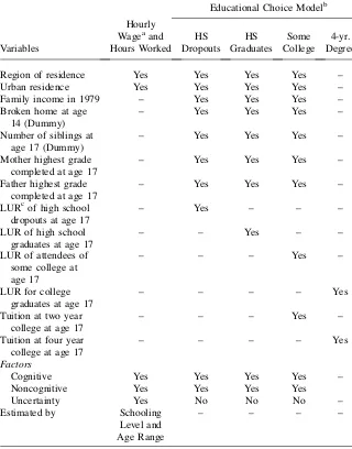
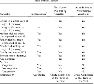
Tables 2a and 2b present the variables included in the empirical implementation of the model, as well as the imposed exclusion and identification restrictions.
VI. Estimation Results
Tables 3 and 4 present evidence on the goodness-of-fit for (log) hourly wages and (log) annual hours worked, respectively. The model does well in predicting the means and standard deviations of hourly wages among whites for any given schooling level and age range (see Panels A and B in Table 3). Formal goodness-of-fit tests cannot reject the null hypothesis that the simulated distributions of hourly wages for whites are statistically equivalent to the actual distributions (Panel C in Table 3). The performance of the model predicting (log) hourly wages for blacks is also good, although some of the goodness-of-fit tests suggest differences between the sim-ulated and actual distributions for high school dropouts and high school graduates.
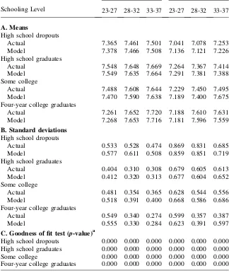
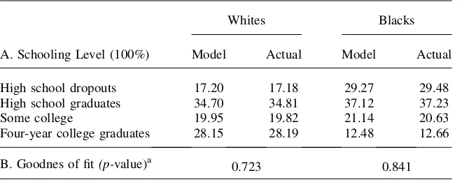
The results for hours worked are not as positive as the ones for hourly wages. Table 4 shows that, even though the model does well in predicting the means and stan-dard deviations of the distributions of hours worked for any given race, schooling level, and age range (Panels A and B), formal goodness-of-fit tests suggest the rejec-tion of the hypotheses of equal distriburejec-tions. However, this result does not have major consequences for the purpose of this paper, since hours worked (in combination with hourly wages) are used to construct annual earnings and, as shown below, the empir-ical model does a good job capturing the observed racial inequality in annual earnings. Tables 5 and 6 analyze the performance of the model in predicting schooling choices, and incarceration rates, respectively. The results from the goodness-of-fit tests show that the model does well in these dimensions for both whites and blacks.
Table 2a
Variables in the Empirical Implementation of the Outcome Equations
Educational Choice Modelb
Region of residence Yes Yes Yes Yes –
Urban residence Yes Yes Yes Yes –
Family income in 1979 – Yes Yes Yes –
Broken home at age
Cognitive Yes Yes Yes Yes –
Noncognitive Yes Yes Yes Yes
Uncertainty Yes No No No –
Estimated by Schooling
Level and Age Range
– – – –
Notes: a. The hourly wage and annual hours worked models are estimated for four different categories (high school dropouts, high school graduates, some college, and four-year college graduates) and for three dif-ferent ranges of age (23-27, 28-32 and 33-37).
b. The educational choice model is estimated considering four different categories: high school dropouts, high school graduates, some college, and four-year college graduates.
It is not possible to reject the null hypothesis that the model produces the same dis-tributions of schooling decisions and incarceration rates as the ones observed in the actual data. These tables also show the substantial racial differences in schooling at-tainment and incarceration rates observed in the data.
Table 2b
Variables in the Empirical Implementation of the model
Measurement System
Variables Incarcerationa
Test Scores (Cognitive Variables)b
Attitude Scales (Noncognitive
Variables)c
Living in a urban area at age 14 (dummy)
– Yes Yes
Living in the south at age 14 (dummy)
– Yes Yes
Mother highest grade completed at age 17
Yes Yes Yes
Father highest grade completed at age 17
Yes Yes Yes
Number of siblings at age 17 (dummy)
Yes Yes Yes
Family income in 1979 Yes Yes Yes
Broken home (dummy) Yes Yes Yes
Age dummies – Yes Yes
Factors
Cognitive Yes Yes No
Noncognitive Yes No Yes
Uncertainty Yes No No
Estimated by Age Range Grade Completed
at the Time of the Test
Grade Completed at the Time of
the Test
Notes: a. There are four models of incarceration, one for each age range (14-22, 23-27, 28-32, and 33-37). Uncertainty is excluded from the model estimated for the first period.
b. Test scores are standardized to have withsample mean 0, variance 1 in the overall population. The in-cluded cognitive variables are Arithmetic Reasoning, Word Knowledge, Paragraph Comprehension, Math Knowledge, Coding Speed, and Numerical Operations;
Table 3
Goodness of Fit - (Log) Hourly Wages by Age Schooling Level, and Race
Schooling Level
Whites Blacks
23-27 28-32 33-37 23-27 28-32 33-37
A. Means
High school dropouts
Actual 2.309 2.387 2.412 2.147 2.185 2.232
Model 2.329 2.402 2.417 2.156 2.201 2.233
High school graduates
Actual 2.436 2.567 2.645 2.198 2.282 2.321
Model 2.435 2.563 2.640 2.204 2.300 2.324
Some college
Actual 2.488 2.691 2.809 2.355 2.460 2.544
Model 2.481 2.686 2.797 2.350 2.438 2.561
Four-year college graduates
Actual 2.524 2.868 3.106 2.482 2.723 2.896
Model 2.539 2.860 3.097 2.448 2.693 2.856
B. Standard deviations High school dropouts
Actual 0.373 0.388 0.455 0.351 0.391 0.424
Model 0.385 0.420 0.488 0.360 0.407 0.436
High school graduates
Actual 0.368 0.402 0.453 0.356 0.388 0.429
Model 0.376 0.419 0.466 0.363 0.392 0.435
Some college
Actual 0.376 0.429 0.517 0.375 0.408 0.407
Model 0.388 0.458 0.564 0.392 0.428 0.450
Four-year college graduates
Actual 0.380 0.437 0.522 0.379 0.454 0.472
Model 0.385 0.445 0.540 0.439 0.532 0.550
C. Goodness of fit test (p-value)a
High school dropouts 0.588 0.766 0.294 0.004 0.009 0.000
High school graduates 0.431 0.448 0.816 0.177 0.014 0.029
Some college 0.143 0.934 0.262 0.055 0.502 0.440
Four-year college graduates 0.157 0.135 0.048 0.437 0.951 0.809
Notes: The simulated data (Model) contains 20,000 observations generated from the Model’s estimates. The actual data (Actual) comes from the NLSY79 sample of Males. For each individual, the schooling level refers to the maximum schooling level reported in the sample.
Table 4
Goodness of Fit - (Log) Annual Hours Worked by Age Range, Schooling Level, and Race
Schooling Level
Whites Blacks
23-27 28-32 33-37 23-27 28-32 33-37
A. Means
High school dropouts
Actual 7.365 7.461 7.501 7.041 7.078 7.253
Model 7.378 7.466 7.508 7.136 7.121 7.226
High school graduates
Actual 7.548 7.648 7.669 7.264 7.367 7.414
Model 7.549 7.635 7.664 7.291 7.381 7.388
Some college
Actual 7.488 7.608 7.644 7.229 7.450 7.495
Model 7.470 7.590 7.638 7.189 7.400 7.675
Four-year college graduates
Actual 7.261 7.652 7.720 7.188 7.610 7.631
Model 7.268 7.653 7.716 7.181 7.596 7.559
B. Standard deviations High school dropouts
Actual 0.533 0.528 0.474 0.869 0.831 0.685
Model 0.577 0.611 0.508 0.859 0.851 0.719
High school graduates
Actual 0.404 0.310 0.308 0.679 0.605 0.613
Model 0.412 0.320 0.313 0.677 0.604 0.652
Some college
Actual 0.481 0.354 0.365 0.628 0.544 0.556
Model 0.518 0.391 0.400 0.668 0.586 0.686
Four-year college graduates
Actual 0.549 0.340 0.274 0.599 0.357 0.387
Model 0.555 0.330 0.284 0.623 0.391 0.597
C. Goodness of fit test (p-value)a
High school dropouts 0.000 0.000 0.000 0.000 0.000 0.000
High school graduates 0.000 0.000 0.000 0.000 0.000 0.000
Some college 0.000 0.000 0.000 0.000 0.000 0.000
Four-year college graduates 0.000 0.000 0.000 0.000 0.000 0.000
Notes: The simulated data (Model) contains 20,000 observations generated from the Model’s estimates. The actual data (Actual) comes from the NLSY79 sample of Males. For each individual, the schooling level refers to the maximum schooling level reported in the sample.
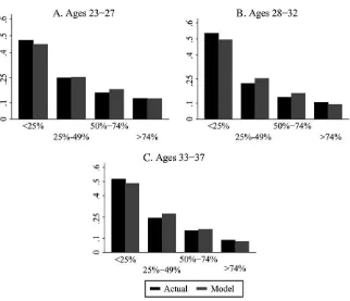
An alternative perspective of the performance of the model is presented in Figures 1 and 2. Figure 1 presents, for each age range, the fraction of blacks reporting hourly wages within different quantiles of the white distribution of wages. The model satisfac-torily mimics the large inequality of wages in the sample. It captures the fact that while approximately 50 percent of blacks report hourly wages that are below the 25th percen-tile of the white distribution, only less than 10 percent of blacks report wages above the 75th percentile of the white distribution. This is consistent across different age groups. Figure 2 repeats the analysis, but for annual earnings. The performance of the model is less satisfactory than in the case of wages, but the model still mimics well the large inequality observed in the data, especially for the last two age ranges.30
Therefore, based on the previous results, it is possible to conclude that the model predicts well the actual racial inequality in labor market outcomes (wages and earn-ings), schooling choices, and incarceration rates.
A. Schooling at Test Date, Observed Test Scores, and Racial Gaps
As explained in Section IVA, this paper treats observed cognitive and noncognitive test scores as the outcomes of a process that has as inputs schooling (at the time tests are taken), family background (mother’s and father’s education, number of siblings, among others), and unobserved abilities. Additionally, the analysis does not constrain the parameters associated with this process to be same across races, so blacks and whites are allowed to have different production technologies of cognitive and non-cognitive test scores. This interpretation of the observed ability measures is formally established in Equations 8 and 9. These equations can be used to analyze the exis-tence of black-white gaps in observed cognitive and noncognitive scores after con-trolling for unobserved abilities and schooling at test date. Additionally, they can be used to study the effect of schooling (at test date) on observed scores (controlling for unobserved abilities), and whether or not this effect differs across races.
Equation 8 is used to construct each of the panels in Figure 3. Each panel shows the significant and positive effect of schooling (at test date) on each of the observed cognitive measures utilized in this paper. The patterns are similar for blacks and whites. It is worth noting that in order to control for the levels of unobserved cogni-tive abilities, the average scores utilized in this figure are constructed assuming the same level of unobserved cognitive ability across races and schooling levels (at test date)ðfW
C ¼fCB¼0Þ, whereas the observable characteristics are set to their respective sample means (black or white sample means). This allows us to distinguish between comparisons of test scores and abilities, controlling for schooling at test date.
In addition to the significant effect of schooling on test scores, Figure 3 also illustrates the sizeable black-white gaps in cognitive test scores. Regardless of the cognitive measure and schooling level considered, on average, whites have signifi-cantly higher test scores than blacks even after controlling for unobserved cognitive ability. The range of values for the computed black-white gaps in test scores is
between -0.5 and -1.5 (recall that the each cognitive test score is normalized to have a mean of zero and a variance of one in the overall population).
The results in Figure 3 also provide new insights about the implications associated with the standard practice of comparing white and black subjects with the same ob-served cognitive test scores. From the analysis of each panel in Figure 3, I can con-clude that, even controlling for the level of unobserved cognitive ability, when we equate blacks and whites on the basis of test scores, we are in fact comparing blacks that have attained substantially more schooling at the test date to whites that have at-tained substantially less. This is particularly important if we consider the significant
Table 6
Goodness of Fit - Incarceration by Age Range and Race
Schooling Level
Whites Blacks
14-22 23-27 28-32 33-37 14-22 23-27 28-32 33-37
A. Fraction of individuals in jail
Actual 1.26 1.87 1.40 1.64 5.31 8.73 12.33 10.53
Model 1.60 1.59 1.09 1.50 7.94 8.31 12.02 10.42
B. Goodness of fit test (p-value)a
0.886 0.959 0.878 0.940 0.359 0.940 0.957 0.896
Notes: The simulated data (Model) contains 20,000 observations generated from the Model’s estimates. The actual data (Actual) comes from the NLSY79 sample of Males. The binary variable Jail takes a value of one if the individual reports at least one episode of incarceration during the respective age range.
a. Goodness of fit is tested using ax2test where the Null Hypothesis isModel¼Data. Table 5
Goodness of Fit - Schooling Choices by Race
Whites Blacks
A. Schooling Level (100%) Model Actual Model Actual
High school dropouts 17.20 17.18 29.27 29.48
High school graduates 34.70 34.81 37.12 37.23
Some college 19.95 19.82 21.14 20.63
Four-year college graduates 28.15 28.19 12.48 12.66
B. Goodnes of fit(p-value)a 0.723 0.841
Notes: The simulated data (Model) contains 20,000 observations generated from the Model’s estimates. The actual data (Actual) comes from the NLSY79 sample of Males.
racial differences in schooling attainment at the time the information on cognitive test scores is collected (see the discussion in Section V).
Figure 4 presents the same analysis but applied to noncognitive measures. The noncognitive scores are also affected by schooling at the time of the test, even after controlling for the level of unobserved noncognitive ability (which is set to 0 across races) and schooling levels. For locus of control (Rotter scale—Panel A in Figure 4), we observe that the gradient of the average score with respect to schooling is larger for whites than for blacks. On the contrary, in the case of self-esteem (Rosenberg Figure 1
Location of Blacks in White Distribution–Hourly Wages Model Versus Data, by Age Range
Note: The panels in this figure compare the proportion of blacks with hourly wages in the respective percentile range of the white distribution obtained using simulated (‘‘Model’’) and actual (‘‘Actual’’) data. The simulated data represents a sample of 20,000 individuals generated from the estimates of the model. The simulated (log) hourly wages are obtained as follows. LetYR
s(a) denote the simulated
individual’s log hourly wage at ageaand schooling levelsgiven individual’s raceR(R={White, Black}). LetDR
s denote a dummy variable that takes a value of one if schooling levelsis selected,
and zero otherwise. Thus, at agea, the individual’s log hourly wage is:
YRðaÞ ¼ +S s¼1
scale—Panel B in Figure 4), the average score for blacks presents the strongest re-sponse to the increase in schooling.
Unlike the case of the cognitive measures, Figure 4 does not show substantial black-white differences after controlling for schooling and unobserved noncognitive abilities. Nevertheless, the comparison of black and white subjects with the same Figure 2
Location of Blacks in White Distribution—Annual Earnings Model versus Data, by Age Range
Note: The panels in this figure present the proportion of blacks with annual earnings in the respective percentile range of the white distribution computed using the simulated (‘‘Model’’) and actual (‘‘Actual’’) data. The simulated data represents a sample of 20,000 individuals generated from the estimates of the model. The simulated earnings are obtained as follows. LetYR
sðaÞandH R
sðaÞdenote the
simu-lated individual’s log hourly wage and log annual hours worked at ageaand schooling levelsgiven individual’s raceR(R¼fWhite, Blackg), respectively. LetDR
s denote a dummy variable that takes a
value of one if the schooling levelsis selected and zero otherwise. Thus, at agea, the individual’s log earning is:
ERðaÞ ¼ +S s¼1
observed noncognitive measures is still problematic. This is because of the signifi-cant racial differences in schooling attainment at the time the noncognitive test scores are collected and because the comparison of the raw scores does not consider the heterogeneity in unobserved noncognitive ability.
In summary, Figures 3 and 4 illustrate the limitations of using observed test scores as proxies for true abilities.
Figure 3
The Effect of Schooling on Observed Measures given fW
C ¼fCB¼0: Black and
White Males
Notes: Each of the observed cognitive measures (test scores) is standardized to have mean zero and variance one in the overall population. Each panel depicts the average cognitive scores computed under the assumption of fW
C ¼fCB¼0. The observable characteristics determining the observed
scores are set to their respective sample means (black or white sample means). Formally, given the schooling level at the time of the test (sT) and race (R), the panel associated with the observed
cognitive measureCipresentsCRiðsTÞ(the mean score) forsT¼ fnine or less years of schooling,
between ten and 11 years of schooling, 12 years of schooling, and some post-secondary educationg
where
CRiðsTÞ ¼uˆRCiðsTÞ+ ˆb R
CiðsTÞXRC+aCiðsTÞ30;
andR¼ fBlack, Whiteg. ˆuR
CiðsTÞand ˆb
R
B. The Distributions of Abilities and Uncertainty
Figure 5 compares the estimated distributions of unobserved cognitive and non-cognitive abilities (Panels A and B, respectively) and uncertainty (Panel C) across races.
Panel A shows that the distribution of cognitive abilities for blacks is dominated by the whites’ distribution. The estimated difference between the means of the white and Figure 4
The Effect of Schooling on Noncognitive Scales given fW
N ¼fNB¼0: Black and
White Males
Notes: Each of the observed noncognitive measures (scales) is standardized to have mean zero and var-iance one in the overall population. Each panel depicts the average noncognitive scores computed under the assumption offW
N ¼fNB¼0. The observable characteristics determining the observed scores are set
to their respective sample means (black or white sample means). Formally, given the schooling level at the time of the test (sT) and race (R), the panel associated with the observed non-cognitive measureNi
presentsNR
iðsTÞ(the mean score) forsT¼ fnine or less years of schooling, between ten and 11 years of
schooling, 12 years schooling, and some post-secondary educationgwhere
NiRðsTÞ ¼uˆRNiðsTÞ+ ˆb R
NiðsTÞXRN+aNiðsTÞ30;
andR¼ fBlack, Whiteg. ˆuR
NiðsTÞand ˆb
R
black cognitive distributions is 0.47, which represents a difference of approximately 1.1 standard deviations.31This difference is consistent with evidence on racial differ-ences in IQ tests reported elsewhere (Jensen 1998; Carroll 1993).32
For noncognitive abilities, the results indicate that, although there are no sig-nificant differences in means, blacks and whites have different distributions of non-Figure 5
Distribution of Unobserved Abilities and Uncertainty by Race
Note: Panel A compares the black and white distributions of unobserved cognitive ability. Panel B compares the distributions of noncognitive ability. Panel C compares the distributions of uncertainty across races. The distributions are computed using 20,000 simulated observations for each race. The simulated data is generated using the estimates of the model.
31. The standard deviations of cognitive ability for whites and blacks are 0.417 and 0.413, respectively. 32. The difference in means is estimated using the logic described for a single cognitive test score in Sec-tion IV.A.1 but applied to all cognitive measures. Specifically, ifDCidenotes the mean difference obtained applying the logic of Section IV.A.1 to test scoreCi, then 0.47 represents the average acrossDC1;.;DCnC wherenCis the number of cognitive test scores. This difference in means is statistically significant at the