A Single-Equation Model and Some Evidence
from French Data
Olivier Donni
Nicolas Moreau
a b s t r a c t
In Chiappori’s (1988) collective model of labor supply, hours of work are supposed flexible. In many countries, however, male labor supply does not vary much. In that case, the husband’s labor supply is no longer informative about the household decision process and individual preferences. To identify structural components of the model, additional information is needed. We thus consider an approach in which the wife’s labor supply is expressed as a function of the household demand for one specific good. We demonstrate that the main properties of Chiappori’s initial model are preserved and apply our results on French data.
I. Introduction
The collective model of labor supply, developed by Chiappori (1988, 1992), is by now a standard tool for analyzing household decisions. This model is based on two fundamental hypotheses—each household member is characterized by specific preferences and decisions result in Pareto-efficient outcomes. These turn out to be sufficient to generate strong testable restrictions on spouses’ labor supply. Moreover, if consumption is purely private and agents are egoistic, the characteristics of the structural model, such as individual preferences and the rule that determines
Olivier Donni is an associate professor of economics at the University of Cergy-Pontoise, THEMA, also affiliated with CIRPEE and IZA. Nicolas Moreau is an assistant professor of economics at the University of Toulouse 1, GREMAQ, also affiliated with IZA. This paper was partly written while Nicolas Moreau was visiting CIRPEE, Universite´ Laval, whose hospitality and financial support are gratefully acknowledged. The authors thank Francxois Bourguignon, Abdel Rahmen El Lahga, and Jean-Marc Robin for useful comments and suggestions. They claim sole responsibility for any remaining errors. The data used in this article can be obtained beginning August 2007 through July 2010 from Nicolas Moreau, Gremaq, Universite´ des Sciences Sociales de Toulouse, Manufacture des Tabacs, Aile J-J Laffont, 21 Alle´e de Brienne, 31000 Toulouse, France. Email: nicolas.moreau@univ-tlse1.fr.
[Submitted May 2005; accepted April 2006]
ISSN 022-166X E-ISSN 1548-8004Ó2007 by the Board of Regents of the University of Wisconsin System
the distribution of welfare within the household, can be identified from the observa-tion of spouses’ labor supply.1
These features of the collective model have turned out to be very attractive, and the number of empirical studies based on Chiappori’s initial framework is considerable. These include Bloemen (2004, Netherlands); Chiappori, Fortin, and Lacroix (2002, United States); Clark, Couprie, and Sofer (2004, United Kingdom); Fortin and Lacroix (1997, Canada); Hourriez (2005, France); Moreau and Donni (2002, France); and Vermeulen (2005, Belgium). However, the large majority of these investigations does not account for the fact that, in most developed countries, male labor supply is rigid and largely determined by exogenous constraints. If the dispersion in husbands’ hours is very limited and/or does not stem from spouses’ optimal decisions, the iden-tification results given in Chiappori’s papers may well be inappropriate.
One important exception in the empirical studies devoted to collective models is given by Blundell et al. (2004). These authors emphasize that in the United Kingdom (but this certainly holds true in other countries), if men work, they work nearly al-ways full-time; the wife’s working hours, on the contrary, are largely dispersed. The theoretical model they develop then allows for these essential features: The wife’s labor supply is assumed continuous, whereas the husband’s choices are as-sumed to be discrete (either full-time working or nonworking). These authors show that the main conclusions derived by Chiappori in the initial context are still valid here. One drawback, however, is that the result of identifiability and testability given by Blundell et al. (2004) holds only if the husband’s choice between full-time work-ing and nonworkwork-ing is free; in particular, it could be seriously misleadwork-ing if involun-tary unemployment is mistakenly interpreted as the decision of not participating in the labor market.
In the present paper, we deal with the rigidity of the husband’s behavior in the French labor market. The approach is quite different from Blundell et al. (2004), though. The starting observation is that the variability in the husband’s working hours is very limited. In addition, since the behaviour of the few husbands who do not work can probably be explained by exogenous constraints (as involuntary unemployment), the employment status of the husband can hardly give reliable information about in-dividual preferences and the decision process. The strategy adopted in what follows is then to exploit the information in household consumption to derive testable restric-tions and identify the intra-household distribution of welfare. However, instead of considering a system of household demands together with the wife’s labor supply, we propose a convenient single-equation approach.2In this approach, the wife’s labor supply is written as a function of her wage rate, other household incomes, sociodemo-graphic variables and the demand for one good consumed at the household level. The
1. The collective model of labor supply has recently been extended in various directions. Chiappori, Blundell, and Meghir (2005) allow for the existence of both private and public consumption. Donni (2003) incorporates the possibility of nonparticipatory decisions and nonlinear taxation. Apps and Rees (1997), Chiappori (1997) and Donni (2005) recognize the role of domestic production and allow for the fact that a proportion of nonmarket time is spent producing goods and services within the household. Fong and Zhang (2001) study a collective model of labor supply where there are two distinct types of leisure: one type is each person’s independent (or private) leisure, and the other type is spousal (or public) leisure. See Vermeulen (2002) and Donni (2008) for a survey of collective models.
idea is that the level of the conditioning good provides information on how the house-hold equilibrium moves along the efficiency frontier when the balance of bargaining power is modified. Indeed, a change in the level of the conditioning good such that the other explanatory variables of the wife’s labor supply remain constant can only be explained by a modification in the spouses’ bargaining power. We then demonstrate that the estimation of this unique equation permits us to carry out tests of collective rationality and identify some elements of the structural model. In addition, we also show that the present framework is compatible with home production if the produc-tion funcproduc-tion belongs to some specific family of separable technologies.
This framework is advantageous on three levels. Firstly, the theoretical results do not postulate a particular explanation for the rigidity of the husband’s behavior. Contrary to Blundell et al. (2004), identification does not exploit the quite limited variations in hus-bands’ working hours, which may well stem from demand side constraints. Secondly, the econometric techniques developed for the estimation of single-equation models can be used to estimate the wife’s labor supply, since the determination of the demand for the conditioning good has not to be explicitly modelled. Thirdly, the variables that af-fect the distribution of power within the household need not be exactly observed be-cause they are summarized by the level of the conditioning good.
These theoretical results are followed by an empirical application using French data for those couples in which the wife participates in the labor market and the hus-band works full-time. The conditioning good is the household expenditures on food at home. The wife’s labor supply is estimated and the restrictions derived from Pareto efficiency are tested. They are not rejected by the data.
The paper is structured as follows. The theoretical model is developed in Section II and a very general functional form is presented in Section III. The data and the em-pirical results are described in Section IV. All the proofs are collected in Appendix 1.
II. Theory
A. Basic Framework
Our theoretical framework is very similar to that used in Chiappori (1988, 1992). We consider the case of a two-person household, consisting of a wifeð Þf and a husband
m
ð Þ, who make decisions about leisure and consumption.3The market labor supply of spousei ið ¼m;fÞis denoted byhi, with market wage ratewi. The consumption is
purely private and —unlike Chiappori’s framework—is arbitrarily broken down into two aggregate goods, which are denoted byciandxi. Each household member is then
characterized by specific preferences overðhi;ci;xiÞ, which can be represented by
utility functions of the form:
uiðThi;ci;xi;zÞ;
ð1Þ
whereT is total time endowment and z is a vector of sociodemographic factors.4 These utility functions are both strongly concave, infinitely differentiable, and
3. The couple is not necessarily married. The terminology is chosen for convenience.
strictly increasing inðThiÞ,ciandxi. The household members are ‘‘egoistic’’ in
the sense that their utility only depends on their own consumption and leisure. This may seem restrictive but, as shown in Chiappori (1992), all the results immediately extend to the case of ‘‘altruistic’’ agents in a Beckerian sense with utilities repre-sented by the form:
Wi umðThm;cm;xm;zÞ;uf Thf;cf;xf;z
;
whereWið Þ is a strictly increasing function. The crucial hypothesis is the existence
of some type of separability in the spouses’ preferences.
At this stage, we suppose that there is no domestic production.5Ifyis the house-hold nonlabor income, the budget set is written as:
y+hmwm +hfwf $c+x
ð2Þ
and
0#hi#T;ci$0;xi$0;
ð3Þ
wherec¼cm+cf andx¼xm+xf. We may note that, in consumer expenditure
sur-veys, consumption is usually recorded at the household level. We thus assume in what follows that the econometrician observeshi,c, andx, but does not observeci
andxi.
In Chiappori’s original contributions, the spouses’ working hours are supposed to vary continuously as a function of both wage rates and household nonlabor income. This is not very satisfying, though. In France—and in many other countries for that matter—the distribution of men’s working hours is very concentrated around the full-time bound. Consequently, as a convenient approximation at least, we assume the husband’s labor supply is constant, that is,
hm¼h;
ð4Þ
where 0,h#T. The reason for this rigidity is beyond the scope of this paper. It may result from the husband’s preferences, demand-side constraints, or institutional rigidities. Quite importantly, however, our theoretical results are general in the sense that they do not rely on a specific explanation of the husband’s behavior.
The main originality of the efficiency approach is the fact that the household deci-sions result in Pareto-efficient outcomes and that no additional assumption is made about the process. That means, for any wage-income bundle, the labor-consumption bundle chosen by the household is such that no other bundle in the budget set could leave both members better off (or more precisely one better off and the other no worse off). This assumption, even if not formally justified, has a good deal of intu-itive appeal. First of all, the household is one of the preeminent examples of a re-peated game. Then, given the symmetry of information, it is plausible that agents find mechanisms to support efficient outcomes since cooperation often emerges as a long-term equilibrium of repeated noncooperative relations. A second point is that axiomatic models of bargaining with symmetric information, such as Nash or Kalai-Smorodinsky bargaining, which have been previously used to analyze negotiation
within the household (Manser and Brown 1980, McElroy and Horney 1981), assume efficient outcomes.
Taking account of the restriction on the husband’s working hours, Pareto-efficiency essentially means that a scalar m exists so that the household behavior is a solution to the following problem:
max
hf;cm;cf;xm;xf
1m
ð Þ uf Thf;cf;xf;z
+mumðThm;cm;xm;zÞ;
ð5Þ
with respect to Equations 2–4. The weightm, which has an obvious interpretation as a ‘‘distribution of power’’ index, is comprised between zero and one. Ifm¼0, the household behaves as though the wife always got her way, whereas, if m¼1, it behaves as if the husband was the effective dictator. The location of the equilibrium along the Pareto frontier will generally be determined by the household characteris-tics (that is,wf;wm;yand z). Hence, using a parameterization, which is convenient
for our purposes, we write:m¼mðwf;c;s;zÞ, wherec¼y+hwmis the ‘‘nonwife’’
income ands¼y=cis the ratio of nonlabor income and nonwife income. To obtain well-behaved labor supplies and demands, we also assume that the function
mðwf;c;s;zÞ is single-valued and infinitely differentiable in all its arguments. The
solutions to the household optimization problem can then be written as cðwf;c;
s;zÞ,xðwf;c;s;zÞ andhfðwf;c;s;zÞ. Note that, in these expressions, the ratio of
nonlabor income and nonwife income affects household behavior only through its impact on the functionm. In standard terminology, such an explanatory variable that does not influence preferences or the budget constraint is called a distribution factor.6
B. Decentralization and Functional Structure
As is well known, if agents are egoistic and consumption is purely private, the effi-ciency hypothesis implies that the household decision process can be represented by a two-stage budgeting problem.7At Stage 1, both spouses agree on a particular dis-tribution of the nonwife incomecbetween them. At Stage 2, each spouse freely chooses his or her level of consumption (and labor supply for the wife), conditional on the budget constraint stemming from Stage 1. Technically, if hf;cm;cf;xm;xf
are solutions to the household problem (Equation 5), a sharingðr;rcÞof nonwife income exists so that the husband’s and the wife’s behaviors can be described by the following individual problems:
A. Husband’s problem:
max
cm;xm
um Thm;cm;xm;z
subject to xm+cm # r; cm $0 andxm$0;
6. Other classical examples of distribution factors, exploited by Chiappori, Fortin, and Lacroix (2002), are given by the state of the marriage market and divorce legislation. Note that in the ‘‘unitary’’ approach to household behavior, where a single utility function is supposed to be maximized by spouses, labor supplies and demands are independent of distribution factors.
B. Wife’s problem:
max
hf;cf;xf
uf Thf;cf;xf;z
subject to xf +cf ¼cr+wfhf;0#hf #T; cf $0 , andxf $0.
In the remainder of the text, the husband’s shareris referred to as the sharing rule. This function can be seen as a reduced form of the balance of power between spouses and, in general, depends on the household characteristics, that is,wf,c,s, andz. We
follow the common practice that supposes these characteristics are given for the household. In doing that, however, we exclude the possibility that individuals choose their own wage rate (through intensity of work or learning effort for instance) to in-fluence their bargaining position in the marriage.8 The reader is referred to Konrad and Lommerud (2000) for a model of strategic determination of wage rates.
The decentralized problems determine the functional structure that characterizes the wife’s labor supply and the household demand for goods. In particular, the wife’s labor supply can be written as:
hf wf;c;s;z
¼hf wf;cr wf;c;s;z
;z
; ð6Þ
whereh is the wife’s Marshallian labor supply, which is obtained from the wife’s problem. This relation satisfies the Slutsky positivity, that is, for an interior solution,
@hf
@wf
@hf
@ðcrÞhf >0: ð7Þ
One important point is that the observation of the sole wife’s labor supply as a function ofwf;c;s;andz is not sufficient to generate testable restrictions or to identify useful
structural components of the model. Indeed, for any observed functionhf wf;c;s;z
and any arbitrary functionhf wf;cr;z
satisfying@hf=@ðcrÞ.0, it is possible to find a functionr wf;c;s;z
such that equality (Equation 6) identically holds. This function is defined by:
r wf;c;s;z
¼ch1f wf;hf wf;c;s;z
;z
;
whereh1
f is the inverse ofhf with respect tocr. Sincehf is arbitrarily chosen,
the sharing rule is not identifiable and the efficiency hypothesis is not testable. Clearly enough, the econometrician must observe a second outcome of the house-hold decision process to obtain interesting results. In his classical model of labor sup-ply, Chiappori (1988, 1992) supposes that the wife’s and the husband’s labor supply are simultaneously observed. In the present framework, since the husband’s labor supply is exogenously determined and tells nothing about the decision process, we shall exploit the observation of the demand for one good.9In particular, the demand for goodx(say) can be written as:
8. We thank an anonymous referee for pointing this out.
x wf;c;s;z
¼zm r wf;c;s;z
;z
+zf wf;cr wf;c;s;z
;z
; ð8Þ
wherezmandzf are the husband’s and wife’s Marshallian demand for goodx respec-tively (conditionally oncr, the functionzmis independent ofwmbecause the
hus-band’s labor supply is fixed). As we shall show, this relation provides information that can be exploited to generate tests and identify structural components of the model.
C. The s-Conditional Approach
In this section, we develop a formulation for the wife’s labor supply that incorporates the information contained in the demand for goodx. To do that, the wife’s working hours are expressed as a function of the wife’s wage rate, the nonwife income, the sociodemographic variables, and the level of goodx. We then show that the obser-vation of this ‘‘conditional’’ labor supply allows us to identify some structural com-ponents of the model and test the efficiency hypothesis.10
The existence of these conditional labor supplies relies on the assumption that the level of goodxis a valid indicator of the ratio of nonlabor income and nonwife in-come. This is formally expressed by the following condition of existence:
@x @s 6¼0; ð9Þ
in an open subset of the domain ofx wf;c;s;z
. In other words, the source of non-wife income (locally) influences the demand for goodx. This condition implies that (i) the spouses’ relative bargaining weightm depends on the source of nonwife in-come, and (ii) the marginal propensity to consume goodxfor the husband and the wife are different.11In particular, if the spouses’ demands for goodxare character-ized by linear Engel curves with the same slope, the demand for goodxat the house-hold level will be independent of the sharing rule and, a fortiori, of the source of nonwife income. This is reminiscent of a well-known result in aggregation theory; see Deaton and Muellbauer (1983), for instance. Empirical evidence suggests, how-ever, that the distribution of exogenous income affects the demand for a large number of different goods.12
If Condition 9 is satisfied, then the demand for goodxcan be inverted onsto yield
s¼s wf;c;s;z
. We incorporate this into the husband’s share of income and obtain what we call the ‘‘s-conditional’’ sharing rule, denoted by
10. Conditional demands or supplies are often used in traditional analysis where a single utility function is assumed; see, for instance, Pollak (1969); Chavas (1984); Browning and Meghir (1991); or Browning (1998). However, the conditional function concerned here is somewhat different.
11. Note also that the conditional labor supplies at stake are not defined in the unitary approach because in that case, household behavior is independent of the source of nonwife income. This should not be a serious problem since the unitary approach was rejected in many studies.
k wf;c;x;z
In this expression, the level of good x can be interpreted as an indicator of the ratio of nonlabor income and nonwife income and, more generally, as a measure of the intrahousehold distribution of bargaining power. For example, if goodxis es-sentially consumed by the wife, that is, the slope of the wife’s Engel curve is greater than that of the husband, then an increase in the wife’s bargaining power will be as-sociated, all other things being the same, with an increase in the household demand for goodx.
Thes-conditional sharing rule differs from the traditional sharing rule in that it has a specific property of separability. This property is described in the following lemma. Lemma 1The s-conditional sharing rule is implicitly defined as the solution of:
x¼zm k wf;c;x;z
The proof is straightforward: For anyk, the equation of demand for goodxmust be identically satisfied. The consequence is that the derivatives of thes-conditional shar-ing rule can be interpreted in terms of the derivatives of the demand for goodx.
Now let us assume that there are no corner solutions. In particular, the wife par-ticipates in the labor market. We then introduce thes-conditional sharing rule into the wife’s labor supply and obtain:
hf wf;c;x;z
This concept will be referred to as the ‘‘s-conditional’’ labor supply.13The structure of this type of labor supply differs from that of the ‘‘unconditional’’ labor supply (Equation 6) in that thes-conditional sharing rulek wf;c;x;z
has a specific prop-erty given in Lemma 1.
The attractiveness of thes-conditional approach ultimately depends on the prop-erties ofs-conditional labor supplies, namely, whether the underlying assumptions are testable and the structural model identifiable from the observation of one
s-conditional labor supply. These important questions are examined in the next section.
D. Properties of s-Conditional Labor Supplies
In order to investigate the testability and identifiability issues we assume that the wife’s s-conditional labor supply exists over an open subsetS. We now introduce some pieces of notation:
In the discussion of Proposition 2 below, we shall show thata wf;c;x;z
can be interpreted as the slope of the husband’s Marshallian demand for goodx(recovered from the derivatives of the s-conditional labor supply), whereasb wf;c;x;z
corre-sponds to the inverse of the derivative of this slope.
Let us assume now that the wife’ss-conditional labor supply satisfies some regu-larity conditions.
Assumption R. The wife’s s-conditional labor supply is such that, for any
wf;c;x;z
The first two conditions mean that the slope of the wife’s Engel curve for the labor supply and that of the husband’s Engel curve for the demand for goodxare different from zero. Note that, if the wife does not participate in the labor market, these con-ditions do not hold, and the conclusions that follow are not valid.
The next result states that thes-conditional sharing rule can be retrieved from the sole observation of the wife’ss-conditional labor supply.
Proposition 2 Let us assume that the wife’s s-conditional labor supply
hfðwf;c;x;zÞsatisfiesR.Then,
(a) thes-conditional sharing rule can be retrieved on S up to a functionkðzÞofz; specifically, its derivatives are given by
@k
(b) for each choice ofkðzÞ, the wife’s marginal rate of substitution between total consumptionðcf + xfÞand leisureðThfÞ, that is, the preferences between total consumption and leisure, is uniquely defined;
(c) the wife’s Marshallian labor supply and the individual Marshallian demands can be retrieved up to a function ofz:
The complete proof of this proposition is given in Appendix 1. We briefly give the first step of the argument here. By definition, the slope of the husband’s Marshallian demand for goodxis given by the increase inxdue to an infinitesimal variation ink, keepingck;wfandzconstant. Note now thathf depends only onck;wf andz.
Then, an infinitesimal variation inc, so thathf,wfandzremain unaffected, provides
the slope of the husband’s Marshallian demand. Consequently, if we apply the im-plicit function theorem tohf wf;c;x;z
such that x is differentiated with respect toc, we obtain the slope of the husband’s Marshallian demand:
@zm
There are two distinct advantages to modelling an s-conditional labor supply instead of one unconditional labor supply and one household demand. Firstly, there is no need to model the determination of the conditioning good explicitly. The
s-conditional approach does not require an explicit structural model for the con-ditioning good at all. In contrast to usual collective models of labor supply, the
s-conditional labor supply can be estimated with single-equation techniques. This is useful because the estimation of labor supply models is generally very expensive in computer-time. Secondly, there is no need to observe the distribution of nonwife income between its sources. This is particularly compelling since, in empirical work, such information is often unreliable. More generally, the effect of any distribution factor, even unobserved or unknown for the econometrician, is incorporated in the conditioning good.
However, thes-conditional approach has also some limitations as far as identifica-tion issues are concerned. Firstly, even if thes-conditional sharing rule can be recov-ered (up to a function ofz), its theoretical interpretation is unclear. The reason is that thes-conditional sharing rule is expressed as a function of the level of goodx, which is endogenously determined. Secondly, the s-conditional sharing rule and the other structural elements can be retrieved as long as the wife participates in the labor mar-ket but the identification cannot be extended beyond the participation set. However, these drawbacks are simply a converse of the fact that we need less information to estimate an s-conditional labor supply than to estimate, as is made in Donni (2007), an unconditional labor supply together with a system of demands. In partic-ular, there is neither a need to observe the level of the demand for goodxwhen the wife does not work, nor one to observe the sources of nonwife income.
We show in the next proposition that the wife’ss-conditional labor supply has to satisfy some constraints to be consistent with collective rationality.
Proposition 3 Let us assume that the wife’s s-conditional labor supply
hfðwf;c;x;zÞsatisfiesR.Then, for anyðwf;c;x;zÞ 2S,
traditional income effect. In particular, the effect of the wife’s share on her labor sup-ply is given by
@h
@ðckÞ¼
@hf=@x
bð@a=@xÞ:
If the condition in Equation b is satisfied, a well-behaved utility function rationalizes the wife’s behavior.
We now suppose that leisure and goods are superior (that is, normal). In many cir-cumstances, this assumption is uncontroversial because goods are very aggregated. If so, the s-conditional approach implies several additional restrictions, which are pre-sented in the next proposition.
Proposition 4 Let us assume that the wife’s s-conditional labor supply hf wf;c;x;z
satisfiesR.Then, for any wf;c;x;z
2S,
(a) if leisure is superior,
@hf=@x
bð@a=@xÞ,0;
(b) ifgoods x and c are superior (for both spouses),
min 1; 1 + 1 +wf @hf=@x
bð@a=@xÞ
.a>max 0; 1
bð@a=@xÞ
:
This result, which is a straightforward consequence of Proposition 2, provides a new test of collective rationality under the additional assumption of consumption superi-ority. In particular, the second statement of Proposition 4 deserves some comments. If one inequality in this statement is violated bya, then (at least) one slope of the four Engel curves must be negative. To illustrate that, let us remember thata coin-cides with the slope of the husband’s Engel curve for goodx. Then, ifa,0, goodx
is inferior for the husband (but goodcis necessarily superior from the Engel’s ag-gregation condition). On the contrary, ifa>1, goodxis superior and goodcis in-ferior. The interpretation of the other inequalities, which are related to the wife’s behavior, is more complicated, though. See the proof in Appendix 1.
E. Another Interpretation: The Role of Domestic Production
Undoubtedly, the absence of domestic production is a serious shortcoming of the model developed above. In this section, we incorporate the fact that a proportion of time not allocated to market labor supply may be spent producing goods within the household. To do so, we suppose thathti¼hi+hdi, whereh
t iandh
d
i respectively
is spousei’s total labor supply and domestic labor supply.14That means, nonmarket time can be broken down into time consumed in leisure,Thti, and time spent in
domestic production,hdi. Then we suppose that goods can be produced using ‘‘indi-vidual’’ technologies of the form:
hdi ¼fi cdi;x
wherefiis a function, increasing and strictly convex in its arguments, andcd i andxdi
denote the proportion of goodscandxentering spousei’s production process, where as usual a positive number indicates an output and a negative number indicates an input. Note that goodsc andx are marketable in the sense that they can either be purchased (or sold) in the market or produced at home.15Also, the prices are exog-enously fixed by the market.
In the specification of the production technology, the fact thatfidoes not depend
onhd
jðj6¼iÞis crucial in the development that follows. That implies there is neither
substitutability nor complementarity in spouses’ time inputs. Overall, this assump-tion seems to be supported (as a valid approximaassump-tion at least) by the rare empirical studies of domestic activities (for example, Graham and Greene 1984). Now let us suppose that spouses’ utility is a function of leisure (instead of nonmarket time) and consumption. We have:
i andxtidenote the proportion ofcandxwhich is ‘‘directly’’ consumed by
spousei (which includes the outputs of the production process and excludes the inputs). We have:cti¼ci +cdi andx
t
i¼xi +xdi, whereciandxidenote the quantity
of goods purchased in the market for spousei’s use.
The basic idea of the reasoning is that if the production technology is of the form of Equation 12, the Utility Function 1, which is used in the preceding sections, can be derived from a more fundamental representation of preferences, described by Equa-tion 13. We have:
Since the price of goods is constant (and equal to one), this result is a straightforward application of the Hicks’ aggregation theorem. The intuition goes as follows. The al-location process can now be represented in three stages. Firstly, spouses agree on a sharing of nonwife income as previously. Secondly, each spouse maximizesuiwith
respect tohi;ciandxi, taking account of the wife’s share of nonwife income. Thirdly,
each spouse maximizesviwith respect tocti;xit;cdi andxdi, taking account of their
in-dividual production technology and their preceding choices ofhi;ciandxi. This last
stage, which characterizes the domestic production interpretation, is described by Equation 14 above. Note that the arbitrage between domestic and market activities is determined by the comparison of market wage rate and domestic productivity.
If productivity is high, it is profitable to devote a large proportion of time to domestic activities. This may explain the specialization of one spouse in market or domestic activities.
Now, if the interpretation above is accepted, the individual demands that are re-trievable from Proposition 2 can be seen as the difference of the demands of goods which are directly consumed xt
i;cti
and those which are produced (or used as inputs) at home xd
i;cdi
. In other words, each demand represents the quantity of goods purchased by spouseiwith her share of nonwife income in the second stage of the decision process described above. In any case, however, the utility functionui,
which is (partially) identified from observed behavior, continues to represent a valid indicator of spousei’s welfare. In addition, the testability results presented in Prop-osition 3 and 4 are still valid in the domestic production interpretation.
III. Parametric Specification of the Model
A. Quadratic Conditional Labor Supply
In order to estimate and test the collective model previously developed we must first specify a functional form for the wife’ss-conditional labor supply. Let us consider a very general, quadratic functional form:
hf ¼a00ðzÞ+a01wf +a02c+a03x+a11w2f +a22c
2+a33x2
+a12wfc+a13wfx+a23cx;
ð15Þ
wherea01;.;a23are parameters anda00is a function of sociodemographic factors. To make things simple, we suppose thata00has a linear form:a00¼a0z, whereais a vector of parameters.
The theory above yields a set of parametric constraints that the functional form (Equation 15) must satisfy. First, from Statement a in Proposition 3, the coefficients of this functional form have to satisfy the following restrictions:16
2a33a12a13a23¼a23a234a22a33¼0: ð16Þ
If these restrictions are imposed, the sharing rule can be retrieved. Moreover, State-ment b in Proposition 3 implies that
a01a03a13
2a33
+ 2 a11 a
2 13
4a33
wf a02
a03a23
2a33
hf >0:
ð17Þ
In principle, this restriction can be globally imposed but it would reduce excessively the flexibility of the functional form. Hence, we prefer checking inequality (Equation 17) for each observation.
B. Recovering the Structural Parameters
Let us defineQ¼a03 +a23c+a13wf + 2a33xandD¼a03a232a02a33. Then the
s-conditional sharing rule is quadratic and its derivatives are given by
@k
Solving this system of three partial differential equations, we obtain thes-conditional sharing rule equation:
whereK0ðzÞis an unidentified function ofz, and where
K1¼
On the other hand, the Marshallian labor supply does not depend on the conditioning goodxand takes the following form:
hf ¼AðzÞ +Bwf +Cw2f +DðcrÞ;
Hence, the wife’s Marshallian labor supply belongs to the family of semi-quadratic specifications, and the normality of leisure implies thatD,0. Note that the utility function that rationalizes this functional form exists in closed form and is given by Stern (1986).
Moreover, if goodsxandcare superior, the slope of the Engel curves generates a strong test of collective rationality, as is explained in the discussion of Proposition 4. To carry out this test, these slopes have to be computed for the present functional form with the identification results given in Proposition 2. However, the formulas are quite complicated, so that the slopes are not exhibited here. Note that the posi-tivity must be checked for each observation since the Engel curves are not linear.
IV. Data and Empirical Results
A. Data
demographic characteristics. We select a sample of married and cohabiting couples where the adults are aged between 20 and 60 and available for the labor market. For this purpose, households where adults are disabled, retired or students are excluded. We also exclude households where adults are self-employed or farmers. The labor supply behavior of these two categories may indeed be rather different from salaried workers and, altogether, would require a different modelling strategy. We further se-lect households where hours of work are positive for wives and at least 35 hours per week for husbands. We also restrict our sample to households with no preschool (un-der three) children in or(un-der to minimize the extent of nonseparable public goods within the household, which is not accounted for in our model. Finally, since Browning and Chiappori (1998) argue that the hypothesis of efficiency in the intra-household decision process is more likely to be satisfied in stable couples, we further restrict our sample to households with at least two years of conjugal life. In all, these selec-tion criteria lead us to 1670 observaselec-tions.
The choice of the conditioning good is a crucial issue that must be discussed. The theory developed above requires the conditioning goodxto be private and nondura-ble. Moreover, as is demanded by Condition 9, the demand for this good must be responsive to variations in the ratio of nonlabor income and nonwife income. Finally, because expenditures on nondurables are recorded in the survey on diaries covering two-week periods (and extrapolated for the year), infrequency of purchases may be a serious issue. We thus choose the household expenditure on food at home (including alcohol and tobacco) as the conditioning good. One advantage of using that variable is that the number of zeros is far lower than for other goods. More importantly, sev-eral studies (Thomas 1993; Hoddinott and Haddad 1995; Phipps and Burton 1998) indicate that the demand for food at home is affected by the fraction of total income controlled by the wife and the husband, respectively.17This is also corroborated by our data. We observe, using a simple reduced-form OLS regression, that the impact of husband’s income on the expenditure on food at home is significantly different from that of nonlabor income. Interestingly, the source of exogenous income does not influence the expenditure on food at home when the regression is based on a sam-ple of single men.18 Be that as it may, to check the robustness of our empirical results, we have also estimated the model with two other conditioning goods, namely, food away from home and clothing. In this case, the collective restrictions (Equations 16 and 17) are not rejected by the data but the coefficients are less precisely esti-mated than with food at home as the conditioning good. These estimations are sum-marized in Table 6 (Appendix 2).
The other variables are defined as follows. The female labor supplyhf is the
num-ber of working hours per week. The wage ratewf is the average hourly earnings
de-fined by dividing the wife’s total labor income on all jobs over annual hours of work on all jobs. As the latter information is not included in the data, it is computed from
hf and the number of months worked during the year. The nonlabor incomeyis
de-fined as the nonlabor income net of savings and is given by the budget identity:
17. The opinion according to which there are some gender-specific differences in many areas of nutrition is also supported by sociologists. For instance, women eat more fruits and vegetables whereas the consump-tion of alcohol, tobacco, fatty foods, and high-sucrose foods is higher in men (Aliaga 2002).
y¼c+xwmhmwfhf, so that the nonwife income cis equal to:c¼c+xm
wfhf. That is, the nonwife incomecis the difference between annual household total
consumption and female labor earnings. In doing that we follow Blundell and Walker (1986) and adjust nonwife income to be consistent with an intertemporally separable lifecycle model. Finally, the sociodemographic factorszinclude the number of chil-dren and the wife’s age.19
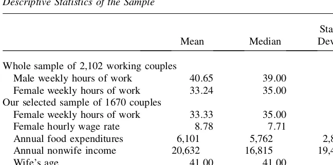
Some descriptive statistics of the sample are exhibited in Table 1. The first and second rows of the table help us compare the distribution of male and female labor supply for working couples. On average, men work more than women do and their labor supply is more concentrated. The comparison with the United States, for in-stance, is striking. In the PSID of 1990, using a similar selection as done here for couples, we find that there is no obvious concentration in the distribution of hours, apart from the mode between 35 and 40 weekly hours. This spike itself concerns only 39.5 percent (36.8 percent) of U.S. men (women) in working couples compared to 65.5 percent (45.9 percent) of the French men (women) in working couples. We are inclined to believe that the variability in husbands’ working hours can simply be disregarded by a study of French wives’ behavior. This issue is examined below with a formal test of the rigidity of male labor supply.
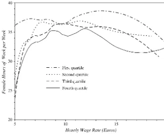
Finally, to have a first look at the form of the wife’s labor supply, we report four locally weighted regressions of female hours on the wage rate in Figure 1. Each line refers to a different quartile of nonwife income. The relationship between hours and wage rates is clearly nonmonotonic and the different curves exhibit a substantial in-come effect. Moreover, for a given wage rate, the slope of these curves depends on Table 1
Descriptive Statistics of the Sample
Mean Median
Standard Deviation
Whole sample of 2,102 working couples
Male weekly hours of work 40.65 39.00 8.09
Female weekly hours of work 33.24 35.00 9.56
Our selected sample of 1670 couples
Female weekly hours of work 33.33 35.00 9.64
Female hourly wage rate 8.78 7.71 4.18
Annual food expenditures 6,101 5,762 2,810
Annual nonwife income 20,632 16,815 19,479
Wife’s age 41.00 41.00 8.15
Number of children 1.28 1.00 1.08
Note: All monetary amounts in euros.
nonwife income. These observations justify our choice of a very flexible specification for the wife’s labor supply.20
B. Endogeneity and Choice of Instruments
The wage rate is computed as labor income divided by hours of work. This may in-duce the so-called ‘‘division bias.’’ Hence, the wage rate may well be endogenous. Moreover, nonwife income and food expenditures are likely to be endogenous as they are choice variables in the model. Therefore, we have chosen to instrument the wife’s wage rate, the nonwife income, the food expenditures and their squares and cross-products. The possible endogeneity of children deserves further attention. On the one hand, we may assume that we only need to worry about the endogeneity of recently born children and can treat older children as predetermined. On the other hand, there is some evidence that labor force behavior surrounding the first birth is a significant determinant of lifetime work experience (Browning 1992). All things con-sidered, this issue is an empirical one. Hence, since the exogeneity of the number of Figure 1
Locally Weighted Regression, FHBS 2000 Data
children is not rejected by our data, the estimations of the model we present below do not instrument the number of children.21
At this stage, the selection of the instruments requires some discussion. First of all, we assume that the wife’s education is not correlated with the error term in the labor supply equation. This assumption, although debatable, is standard in the labor supply literature (see, among others, Bourguignon and Magnac 1990; Blundell et al. 1998; Chiappori, Fortin, and Lacroix 2002; and Pencavel 1998). The wife’s education is a convenient in-strument for her wage rate. In addition, the growth of wage rates along the lifecycle is generally a function of education. Thus, we also use as instruments a second order poly-nomial in age and education for the wife. This gives four excluded instruments (account-ing for the fact that the wife’s age is a control variable in the labor supply equation).
The various sources ofexogenousincomes are natural instruments for the nonwife income and the food expenditures. In particular, since the husband’s labor supply is exogenously constrained, we may suppose that the husband’s annual labor earnings is exogenous.22 Then, to grasp as much variation as possible in the endogenous regressors, we use a fourth-order polynomial in the husband’s labor earnings and ob-tain four extra instruments. We also use a second order polynomial in exceptional incomes (including inheritance, bequests, and gifts) as instruments.23
Other instruments include a second-order polynomial in age and education for the husband (five instruments), two dummies for husband’s father’s profession, a dummy variable for living in the Paris region and a cross-term of wife’s education and hus-band’s labor earnings. Our intuition is that these variables have an impact on the var-ious sources of the household income. As usual, measurement error in the instruments is not supposed to be correlated with the response error for the endogenous variables.24 All in all, there are four included instruments (a constant, the wife’s age, the num-ber of children, and the inverse of Mill’s ratio) and 19 excluded instruments from the labor supply equation. In the next section, we shall check the validity of some of our exclusion restrictions.
C. Results
Before we present any further results, we report the tests of the validity of the instruments.
1. The Validity of the Instruments
We first test the null hypothesis that none of the excluded instruments is correlated with the endogenous variables in the system of equationsY¼WG+e, whereYis the matrix of endogenous regressors,Wthe matrix of instruments, andGa matrix
21. However, our conclusions are still valid when the number of children is supposed to be endogenous. In that case, the estimates differ only in that the coefficient of the number of children in the functional form (Equation 15) is no longer significant. These results are available upon request.
22. The husband’s wage rate may be endogenous, though. This issue is examined in greater details in sec-tion IVC3.
23. To avoid strongly correlated instruments, we replace the polynomials with their corresponding princi-pal components, that is, with orthogonal linear combinations of the original instruments. Estimates are then more stable.
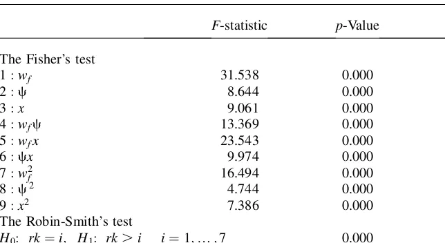
of parameters andea matrix of random terms. The first panel of Table 7 in Appen-dix 3 showsF statistic, correspondingp-value and adjustedR-square for each of the nine auxiliary regressions. Thep-values are close to zero, indicating that the null hypothesis is clearly rejected. This gives evidence that the instruments are significant for all the endogenous variables. Note, however, that theFstatistic concerning the aux-iliary regression onc2is relatively small (less than 5). In a 2SLS context, Staiger and
Stock (1997) suggest that estimates and confidence interval may be unreliable with first-stageF’s this small.25On the other hand, Bound, Jaeger, and Baker (1995) mention that results should be interpreted with caution for first-stageFstatistics close to one. To decide on the potential weakness of our instruments, we test whether the ex-cluded instruments have enough explanatory powerjointly for all the endogenous variables. For that purpose, we use the test provided in Robin and Smith (2000). This test evaluates the rank of the coefficient matrix on the excluded instruments in the auxiliary regressions. LetL^ be a consistent and asymptotically normal estimator of ap3k reduced form parameter matrixL on the excluded instruments.26Here we havep¼19 excluded instruments andk¼9 endogenous variables. IfLis not full rank (that is,rkðLÞ,9), the excluded instruments are weak for at least one en-dogenous variable. If L is full rank (rkðLÞ ¼9), the excluded instruments have enough explanatory power jointly for all the endogenous variables. The Robin-Smith test of rank is based on the Eigen values ofL^TL.
Following the sequential procedure advocated in Robin and Smith (2000), we test forH0: rkðLÞ ¼ragainstH1: rkðLÞ.rforr¼1;.;9 and halt at the first value ofrfor which the test statistic indicates a nonrejection ofH0. The second panel of Table 7 in Appendix 3 exposes the results. Again, thep-values are close to zero. The null hypothesis rkðLÞ ¼1 is rejected, so is the null rkðLÞ ¼2, and so on until
rkðLÞ ¼8 is also rejected: The reduced form coefficient matrixLis full rank. We thus conclude that the excluded instruments are valid enough to give reliable esti-mates and confidence interval.
Finally, we consider whether Paris region, female education, and unemploy-ment rates (which appear in the selection equation; see Appendix 3) are valid exclusion restrictions. Including the Paris region or the unemployment rates var-iables in the labor supply equation does not have significant effects on the orig-inal parameters estimates. Thet-value for the coefficient of the Paris region is below 1.2 whereas thet-values for the unemployment rates variables are below 0.4. We hence maintain these exclusion restrictions. If we allow the wife’s edu-cation level to appear in the labor supply equation, it is statistically significant but the estimates of the parameters of interest change and become very imprecise. In fact, the first-stageF’s of the auxiliary regressions related to her wage rate de-crease substantially. When her education level is not excluded from her labor supply equation, her wage rate is weakly instrumented. We therefore maintain this exclusion restriction.
25. We allow for heteroskedasticity of unknown form. We do not know whether these differences signif-icantly affect their asymptotic or not.
2. Labor Supply Estimates
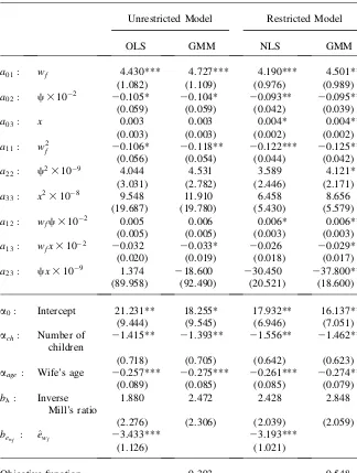
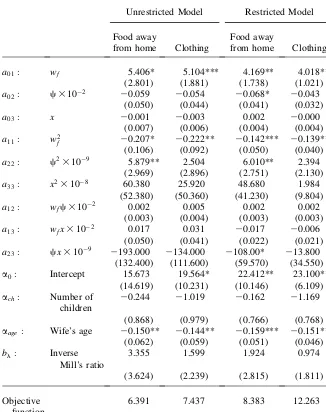
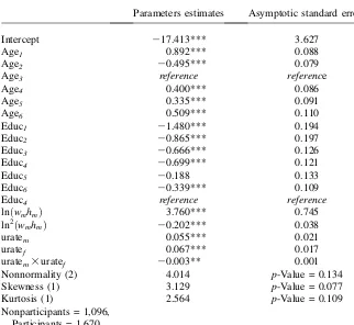
Conditioning the sample on stable households with working wives and no children under three years of age may induce a selectivity bias. To account for these selection rules we estimate a reduced-form participation equation and compute the inverse Mill’s ratio.27The latter is denoted by^land the matrix of residuals obtained from the regression of the variables on the instruments (that is,Y¼WG+e) by^e. Then the first and third columns of Table 2 provide estimates of the unrestricted and re-stricted models obtained by applying OLS (NLS) on the following relation:
hf ¼gðwf;c;x;z;aÞ+^lbl +^ebe +v;
ð20Þ
wheregðÞis the functional form (Equation 15) of the wife’s labor supply,vis a ran-dom term that represents the unobserved heterogeneity, anda;bl, andbe are
param-eters. The inclusion of the residuals in the labor supply equation is to control for the endogeneity of the regressors.28Thet-statistics of the estimates ofbealso provides a
direct test of exogeneity; see Smith and Blundell (1986), or Blundell, Duncan, and Meghir (1998) for a recent application. To save space, only the test of exogeneity for the wife’s wage rate is reported in Table 2. The residual of the regression of the wife’s wage rate on the instruments is denoted bye^wf. Then, under the null
hy-pothesis, the parameterbewf corresponding to the residual^ewf in Equation 20 must be
equal to zero. This is clearly rejected by the data. The wage rate has to be instru-mented.
The second and fourth columns of Table 2 are the unconstrained and constrained models obtained by using GMM on the following equation:
hf ¼gðwf;c;x;z;aÞ+^lbl +v:
ð21Þ
The Hansen’s test does not reject the validity of the instruments and the overidenti-fying restrictions. The test statistics 9.393 and 9.548 are less than the critical values of thex2
0:05ð10Þ ¼18:307 and of thex20:05ð12Þ ¼21:026.
Let us take a closer look at the results of Table 2. Except for the interaction term
c3x, the OLS and GMM estimations give similar results. Since the GMM estimator attains greater efficiency under the presence of heteroskedasticity of unknown form (Davidson and MacKinnon 1993, p. 599), we only refer to the GMM results in what follows.
To begin with, we note that the parameters of the unrestricted model are not esti-mated with precision. Only the wife’s age, the number of children, the wage rate, its square, its interaction with food expenditures and the nonwife income have an im-pact at the 5 percent or 10 percent level. This lack of precision can be explained
27. The estimates of the selection equation are shown in Table 8 (Appendix 3).
28. The asymptotic covariance matrix is computed using the results of Newey (1984) and Newey and McFadden (1994) to take into account that we are conditioning on generated regressors (that is,^land
^
e). This matrix is robust to heteroskedasticity of unknown form and the covariance of the coefficients^G
Table 2
Estimated Parameters of the Reduced Form Labor Supply
Unrestricted Model Restricted Model
OLS GMM NLS GMM
a01: wf 4.430*** 4.727*** 4.190*** 4.501***
(1.082) (1.109) (0.976) (0.989)
a02: c3102 20.105* 20.104* 20.093** 20.095**
(0.059) (0.059) (0.042) (0.039)
a03: x 0.003 0.003 0.004* 0.004**
(0.003) (0.003) (0.002) (0.002)
a11: w2
f 20.106* 20.118** 20.122*** 20.125***
(0.056) (0.054) (0.044) (0.042)
a22: c2
3109 4.044 4.531 3.589 4.121*
(3.031) (2.782) (2.446) (2.171)
a33: x23108 9.548 11.910 6.458 8.656
(19.687) (19.780) (5.430) (5.579)
a12: wfc3102 0.005 0.006 0.006* 0.006**
(0.005) (0.005) (0.003) (0.003)
a13: wfx3102 20.032 20.033* 20.026 20.029*
(0.020) (0.019) (0.018) (0.017)
a23: cx3109 1.374 218.600 230.450 237.800**
(89.958) (92.490) (20.521) (18.600)
a0: Intercept 21.231** 18.255* 17.932** 16.137**
(9.444) (9.545) (6.946) (7.051)
ach: Number of children
21.415** 21.393** 21.556** 21.462**
(0.718) (0.705) (0.642) (0.623)
aage: Wife’s age 20.257*** 20.275*** 20.261*** 20.274***
(0.089) (0.085) (0.085) (0.079)
bl : Inverse
Mill’s ratio
1.880 2.472 2.428 2.848
(2.276) (2.306) (2.039) (2.059)
bewf : ^ewf 23.433*** 23.193***
(1.126) (1.021)
Objective function 9.393 9.548
by the flexibility of our functional form. Nonetheless, the coefficients of the re-stricted model (that is, with the imposition of Condition 16) are very similar, but ex-hibit smaller standard errors, so that most of them are statistically significant at the 5 percent or 10 percent level. In particular, the wife’s age and the number of children have a significant, negative effect on the number of working hours.
We now turn to the test of the collective restrictions. First, we perform a Newey-West’s test of Condition 16. Since the difference in the function values (9:548
9:393¼0:155) is much smaller than the critical value,x2
0:05ð Þ ¼2 5:99, we do not
reject the restrictions at stake. However, this evidence in favor of the collective model must be interpreted with caution. Indeed, the standard error of the coefficient
a33is large. Since this coefficient enters conditions (Equation 16), the test we carry out is not likely to be powerful.
Using the estimates of the restricted model, we note that the Slutsky Condition 17 is satisfied for a large majority (93 percent) of the households in the sample, and the wife’s leisure is superior.29
These results support the collective model and they will be more closely exam-ined below. In addition, the positivity of the slopes of the Engel curves can be checked since it is reasonable to assume that both goods are superior. This corre-sponds to a test of the second statement in Proposition 4. Actually, we observe that the slopes of the four Engel curves are positive for 95 percent of the households in the sample. This confirms that the goods are superior and, incidentally, validate our estimations.
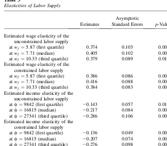
On the whole, the empirical tests we describe above do not reject the collective model. We now consider the various labor supply elasticities that are shown in Table 3. The elasticities of the constrained and unconstrained models are similar and quite precisely estimated. Women’s wage elasticities are positive and statistically signif-icant. Income elasticities are negative and also statistically signifsignif-icant. The ampli-tude of these figures is somewhat different from that found in other studies using French data. For example, estimating a unitary model that accounts for nonlinear taxation and nonparticipation, Blundell and Laisney (1988) report, at the sample mean, wage and income elasticities, which are equal to two and -0.7, respectively. According to the specification used, these elasticities range from 0.05 to one respec-tively and from -0.3 to -0.2 in Bourguignon and Magnac (1990). The elasticities pre-sented in Table 3 differ from previous estimations because our sample is restricted to working wives.
The estimation of the reduced form parameters allows us to retrieve some struc-tural components of the model. The first panel of Table 4 reports the estimates of the parameters of the Marshallian labor supply (Equation 19). The coefficients have the expected signs but the effect of the wife’s share of income is imprecisely esti-mated. Note also that the wife’s Marshallian labor supply is backward bending. For small values of the wife’s wage rate, the substitution effect dominates the income effect so that an increase in the wife’s wage rate has a positive impact on the working hours. For large values of the wife’s wage rate the converse is true. Then the rejection of Slutsky positivity appears for some households in which the wife is characterized
by a very large wage rate. The second panel of Table 4 includes the wage elasticity conditional on the sharing of nonwife income. This ignores any effect the wage rate may have on the intra-household decision process. We note that the wage elasticity is positive, concave, and statistically significant at the 10 percent level. Its value is twice as big as those reported in Table 3 and is close to one at the mean of the sam-ple. It is noteworthy that this figure may be compared with what is found in the lit-erature on collective models. For example, Chiappori, Fortin, and Lacroix (2002) report a wage elasticity of 0.178 with United States data, Fortin and Lacroix (1997) a wage elasticity of 0.361 with Canadian data, and Moreau and Donni (2002) a wage elasticity of 0.394 with French data. The elasticities in Table 4 are substantially greater. However, they are compatible with previous researches since the standard errors of the estimated parameters are quite large.
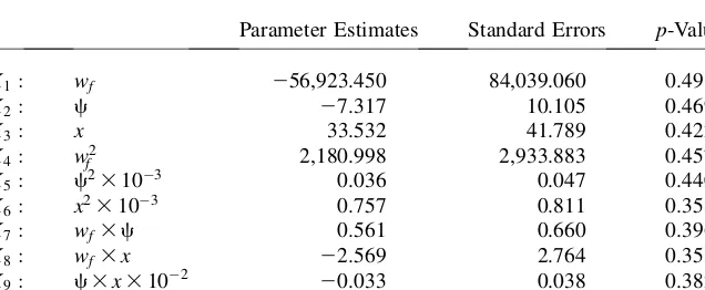
Finally, the sharing rule estimates are shown in Table 5. The parameters turn out not to be precisely estimated: no coefficient is significant at the 10 percent level. We finally compute the marginal impacts of the exogenous variables on the sharing rule (these are not reported here) but none of them is significant.
Table 3
Elasticities of Labor Supply
Estimates
Asymptotic
Standard Errors p-Values
Estimated wage elasticity of the unconstrained labor supply
at wf ¼5:87 (first quartile) 0.374 0.103 0.000
at wf ¼7:71 (median) 0.405 0.102 0.000
atwf ¼10:33 (third quartile) 0.379 0.089 0.017
Estimated wage elasticity of the constrained labor supply
at wf ¼5:87 (first quartile) 0.386 0.086 0.000
at wf ¼7:71 (median) 0.416 0.088 0.000
atwf ¼10:33 (third quartile) 0.384 0.083 0.000
Estimated income elasticity of the unconstrained labor supply
at c¼9842 (first quartile) 20.143 0.057 0.012
at c¼16815 (median) 20.217 0.084 0.009
at c¼27341 (third quartile) 20.286 0.106 0.007
Estimated income elasticity of the constrained labor supply
at c¼9842 (first quartile) 20.136 0.049 0.006
at c¼16815 (median) 20.207 0.074 0.005
at c¼27341 (third quartile) 20.276 0.098 0.005
3. Tests of Husband’s Labor Supply Rigidity
Our theoretical results crucially rely on the postulate that the wife’s labor supply is independent of the husband’s wage rate (conditionally on the levels of nonwife income and one reference good). This is a consequence of the husband’s labor supply rigidity. In particular, if the husband’s hours of work vary, the wife’s labor supply will in general depend on the husband’s wage rate. In that case, our conclusions will be invalidated.
As a matter of fact, the data indicate that the dispersion of the husband’s working hours is quite limited. In spite of that, the husband’s wage rate can possibly influence the wife’s behavior and question the validity of our approach. Also, the rigidity of the husband’s behavior must be tested. To do that, we introduce an additional term,wm,
in the functional form (Equation 15) and assess its significance.30We perform this test whetherWmis included or not in the set of instruments, whereWmis the matrix
of variables constructed from the husband’s labor income. In both cases, the hus-band’s wage rate has no impact statistically different from zero.
We also test in the estimation of Equation 15 for the endogeneity of the subset of instrumentsWm. Suppose that the husband’s wage rate is exogenous. Now it is
or-thogonal to the error term if husband’s labor supply is exogenously constrained. Oth-erwise, it is not. The corresponding test statistic is simply the difference in the criterion functions for GMM estimation with and without the questionable instru-mentsWm (Ruud 2000, p. 576). Under the null hypothesis of orthogonality it
con-verges in distribution to a x2ðkÞ random variable, where k¼5 is the number of
questionable instruments. The difference gives a test statistic of 8.139 (8.115 if the collective restrictions (16) are imposed). At conventional levels we do not reject the null hypothesis.31 In conclusion, even if the husband’s working hours exhibit some dispersion, this should not prevent us from applying the present theory. In Table 4
Estimated Parameters of the Structural Model: The Marshallian Labor Supply
Parameters
Asymptotic
Standard Errorsp-Values
B: wf 11.011 6.187 0.075
C: w2
f 20.374 0.235 0.111
D: ðcrÞ3102 20.011 0.013 0.368
Estimated wage elasticity of the Marshallian labor supply
athf ¼39, withwf ¼5:87 (first quartile) 0.996 0.529 0.060
athf ¼39, withwf ¼7:71 (median) 1.035 0.537 0.054
athf ¼39, withwf ¼10:33 (third quartile) 0.868 0.449 0.053
Note: Asymptotic standard errors are computed with the Delta method.
30. This procedure is intended to test the implication of the dispersion in husband’s hours that may inval-idate our theory.
addition, this test reinforces the evidence that the husband’s labor supply is exoge-nously determined in France.
V. Conclusion
In the present paper, we suppose that the husband’s labor supply is exogenously determined. We then advocate a simple approach to model the wife’s labor supply, in which the wife’s behavior is explained by her wage rate, other house-hold incomes, sociodemographic variables, and the demand for one good consumed at the household level. In this approach, the level of the conditioning good can be interpreted as an indicator of the distribution of power within the household.
We then demonstrate that the estimation of a single equation (including one con-ditioning good as argument) permits to carry out tests of collective rationality and to identify some elements of the structural model. The simplicity of the estimation method suggests that the approach used in this paper is especially profitable to per-form empirical tests.
Another important contribution of the present paper is to show that our approach (and the collective setting as a whole for that matter) is compatible with domestic production on the condition that the household production function belongs to some specific family of separable technologies.
Finally, these theoretical considerations are followed by an empirical application using a French sample of working wives. We show that, overall, the collective restrictions are satisfied by the data. However, the estimates of the structural model are not precisely estimated. One way of dealing with that is to exploit the information on nonparticipating wives.
Indeed, the parameters that enter the ‘‘reduced’’ participation equation (used in constructing the inverse Mill’s ratio) are not related to the parameters of the labor supply equation. In that case, the basic idea is to estimate a ‘‘structural’’ participation Table 5
Estimated Parameters of the Structural Model: The Sharing Rule
Parameter Estimates Standard Errors p-Value
K1: wf 256,923.450 84,039.060 0.498
K2: c 27.317 10.105 0.469
K3: x 33.532 41.789 0.422
K4: w2
f 2,180.998 2,933.883 0.457
K5: c2
3103 0.036 0.047 0.440
K6: x2
3103 0.757 0.811 0.351
K7: wf3c 0.561 0.660 0.396
K8: wf3x 22.569 2.764 0.353
K9: c3x3102 20.033 0.038 0.382
equation, derived from the comparison of a shadow wage equation (incorporating the parameters of the wife’s labor supply) and a market wage equation. The implemen-tation of this idea raises some econometric difficulties, though. This is the topic of future work.
Appendix 1
Proof of Propositions
A. Proof of Proposition 2
In what follows, we first demonstrate Statements a and c of Proposi-tion 2; we then demonstrate Statement c.
Identification of@z=@k. Differentiating the s-conditional labor supply with respect tocandxgives:
Similarly, using Lemma 1 and differentiating the household demand for goodxwith respect toxandcgives:
1¼ @zm
Substituting Equation 22 into Equation 25 yields the husband’s Engel curve:
@zm
Identification of@k
Since
this system of partial differential equations, together with Equation 22, can be solved with respect to@k
s-conditional labor supply with respect toxandwf, we obtain:
@hf
Sinceb6¼0 and @a=@x6¼0, substituting Equation 27 into Equation 28 yields:
@hf
Identification of@zf
@ðckÞ and@zf
@wf. The slopes of the demand for goodx
can be retrieved in a similar way. Substituting Equations 26 and 27 into Equation 23 gives:
Differentiating the household demand for goodxwith respect towf, and using
Equa-tions 26 and 27 yields:
@zf
Identification of other elements. The derivatives of the Marshallian demands for good
ccan be obtained from the individual budget constraints. Moreover, once the function
kðzÞis picked up, the wife’s total consumption can be retrieved. Then, the wife’s utility function is derived as usual; see Deaton and Muellbauer (1983) for instance.
B. Proof of Proposition 3
1. Substituting Equation 29 into Equation 7 yields:
@hf
2. From Young’s Theorem, the derivatives of the sharing rule have to satisfy a symmetry restriction. Using Statement a in Proposition 2 and simplifying yield:
C. Proof of Proposition 4
(a) From Equation 29,
@hf
@x
bð@a=@xÞ.0;
if wife’s leisure is normal. This gives the first statement in Proposition 4. (b) From Equations 26 and 30,
a>0;a 1
bð@a=@xÞ.0;
if goodx is normal (for both spouses). From these expressions and the individual budget constraints, we obtain:
1@zm
@k ¼1a>0;
1 @zf @ðckÞwf
@hf
@ðckÞ¼1a+
1 +wf @hf
@x
bð@a=@xÞ .0;
if goodcis normal (for both spouses). Rearranging these expressions gives the sec-ond statement.
Appendix 2
Alternative Estimations
We carry out two alternative estimations of the model, with expenditures on food away from home and clothing as the conditioning good respectively. One problem, however, is that reported expenditures on clothing (food away from home) are equal to zero for 7.5 percent (18 percent) of the 1670 households of our selection. Be that as it may, these estimations are presented in Table 6. For the sake of comparability, the estimated parameters are obtained with the same set of instruments as those used for the regression in the main text. To complete these results, note that the parameters
BandCof the Marshallian labor supply are significant at the 1 percent level when the conditioning good is food away from home; in that case, the parametersK6and