Implications for Fertility and
School Enrollment
Prashant Bharadwaj
Bharadwajabstract
Does the postponement of marriage affect fertility and investment in human capital? I study this question in the context of a 1957 amendment to the Mississippi marriage law that was aimed at delaying the age of marriage; changes included raising the minimum age for men and women, parental consent requirements, compulsory blood tests, and proof of age. Using a difference- in- differences design at the county level, I fi nd that, overall, marriages per 1,000 in the population in Mississippi and its neighboring counties decreased by nearly 75 percent; the crude birth rate decreased between 2 and 6 percent; and school enrollment increased by 3 percent after the law was enacted (by 1960). An unintended consequence of the law change was that illegitimate births among young black mothers increased by 7 percent. I show that changes in labor market conditions during this period cannot explain the changes in marriages, births, and enrollment. I conclude that stricter marriage- related regulations that lead to a delay in marriage can postpone fertility and increase school enrollment.
I. Introduction
The decision of when to marry has important consequences for men and women. Particularly for women, early marriage is often associated with lower socioeco-nomic status and less schooling (Dahl 2009, Field and Ambrus 2006). Marital status is also known to be an important determinant of female labor force participation (Angrist and Evans 1996, Heckman and McCurdy 1980, Stevenson 2008); moreover, women seem to invest more in their careers if they delay fertility and marriage (Goldin and Katz 2002). It is clear that women’s (and to some extent men’s) marital decisions are intricately tied to their economic outcomes. While marriage is considered a choice, laws
regard-Prashant Bharadwaj is an assistant professor of economics at the University of California San Diego. He thanks Achyuta Adhvaryu, Joseph Altonji, Michael Boozer, Gordon Dahl, Roger Gordon, Fabian Lange, Paul Niehaus, and Ebonya Washington for comments on earlier versions of this paper. Dick Johnson was instrumental in obtaining historical data from Mississippi. Hrithik Bansal, Karina Litvak, and Taylor Marvin provided excellent research assistance. Data used in this paper are available from the author from October 2015 through September 2018 at prbharadwaj@ucsd.edu.
[Submitted August 2010; accepted July 2014]
ISSN 0022- 166X E- ISSN 1548- 8004 © 2015 by the Board of Regents of the University of Wisconsin System
ing marriage often control various aspects of who marries, when people marry, partner choice, and number of partners. Moreover, societal norms place importance on the act of marriage to legitimize cohabitation and childbearing. In the United States, for example, married couples form 90 percent of all heterosexual couples (U.S. Census Report 2007),1
and the majority of children are born to married couples (Hamilton et al. 2005). Given the central role of marriage (78 percent of all women older than 18 marry), marriage laws can have direct implications for the economic outcomes of men and women.
Marriage laws can be used as a policy tool as well—in 1980, China raised the age of marriage for women in a bid to control fertility. On the other hand, if legal marriage is just a formality or if marriage laws are routinely ignored,2 then it is likely that changes
in marriage law will not have much of an impact. Given the intended policy goals of marriage laws as well as rising cohabitation rates, an important empirical question sur-rounding marriage laws is whether changes in marriage laws, particularly changes that raise the cost of marriage, have an impact on marriage rates, fertility, and schooling. Fertility and schooling refl ect key investments that men and women make early in their adult lives that have long- term consequences for welfare and labor market outcomes; hence, from a policy perspective it is relevant to know whether and how marriage laws affect these investments. Although many recent papers have examined the con-sequences of divorce laws,3 few have studied the impact of marriage law changes on
outcomes such as fertility and schooling. Dahl (2009) uses marriage law changes as an instrument for delayed marriage to study the relationship between early teen marriage and poverty. However, Dahl uses marriage law changes along with schooling changes to analyze the impact of both laws simultaneously as changes in compulsory schooling laws often coincide with changes in marriage laws. Buckles, Guldi, and Price (2009) examine the role played by blood test requirements for obtaining marriage licenses, and they fi nd that even small increases to the cost of marriage can decrease marriage rates and increase the incidence of illegitimate births. Finally, Blank, Charles, and Sallee (2009) fi nd evidence of misreporting of age in marriage licenses, and they also fi nd that young men and women tend to avoid restrictive marriage laws by getting married in a different state. This paper adds to this body of work by examining not only the effect of changes in marriage laws on marriage rates but also on fertility and educational invest-ments. While this paper examines the impact of a wide range of marriage law changes, the results make it clear that the age restrictions perhaps have the largest impact. Hence, this paper complements Buckles, Guldi, and Price (2009) in showcasing another aspect of marriage law changes and its impact on a wide range of policy relevant outcomes.
A priori, it is not clear what effect increasing barriers to marriage will have on fertil-ity and schooling. If entering into marriage becomes harder, individuals simply may have children out of wedlock, exacerbating the problem since then the father is less
1. While rates of cohabitation have been on the rise in the United States, demographic evidence suggests that it is not becoming a substitute to marriage (Raley 2001).
likely to help raise the child. After marriage, the sharing of resources becomes easier; hence, spouses may also be more likely to have a chance to get further education. So, the postponement of marriage could reduce education (Stevenson 2007 shows that divorce laws negatively impact spousal support for education- related investments). Alternatively, if people are reluctant to have children out of wedlock, postponement of marriage could lead to a drop in the birth rate. Moreover, unmarried women lacking spousal support might have more incentives to invest in their own education. There-fore, marriage laws could increase school enrollment and educational attainment; the impact of changes in marriage law is essentially an empirical question.
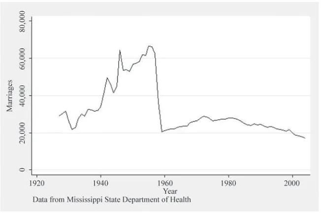
In 1957, the state of Mississippi amended its marriage law. Although the marriage law amendment was passed in 1957, it went into effect in 1958 and immediately resulted in a substantial decline in marriages performed in Mississippi (see Figure 1). The changes included an increase in the minimum marriage age for women from 12 to 15 years old and for men from 14 to 17 years old. The law also introduced a parental consent requirement if either party was younger than 18, a compulsory three- day waiting period, serological blood tests, and proof of age. In addition, brides under the age of 21 were required to marry in their county of residence. Hence, the barriers to marriage were raised not just via increasing minimum age laws but also by introducing blood tests and other requirements, which affected everyone. Using a difference- in- differences strategy that considers Mis-sissippi and its surrounding counties as the treatment group and remaining counties in the states neighboring Mississippi (Alabama, Louisiana, Arkansas, and Tennessee) as the con-trol group, I fi nd that by 1960 marriages per 1,000 decreased by 75 percent, the crude birth rate (births per 1,000 in the population) decreased between 2 and 6 percent, and enrollment among 14–17- year- olds increased by 3 percent more than the corresponding change in the control group. Using yearly state- level data from 1952 to 1960, I fi nd that the percent-age of total births to young black women decreased by 8 percent; for white women, the decline was 18 percent more than the change in the control group. However, this decrease in births is mitigated by an increase in illegitimate births, primarily among black women.
I focus on short- run effects of the law change as there were tremendous social and eco-nomic changes in the 1960s—particularly due to the Civil Rights Act of 1964—that could confound an analysis of long- run outcomes. Moreover, the 1960s and 1970s saw the introduction of various contraceptives (the birth control pill in particular), the legalization of abortion, and changes in divorce laws, which could also affect marriage and fertility (Goldin and Katz 2002, Donohue and Levitt 2001, Ananat and Hungerman 2007, Bailey 2006). With this caveat in place, using the 1990 census, I do not fi nd long- run effects on fertility, suggesting that the drop in birth rates is simply a delay in fertility.4 I do
fi nd that women affected by the law were more likely to complete high school in the long run.
This paper’s relevance extends to the context of developing countries, where age at
fi rst marriage and educational attainment of women tend to be quite low. Therefore, for women in developing countries who have high levels of fertility and low levels of educa-tional attainment, laws that delay marriage might be welfare improving. Field and Ambrus (2008) show that women who marry later attain more years of education in Bangladesh. Given this fi nding, they hypothesize that imposing universal age of consent laws can raise educational levels of women. The fi ndings of this paper provide direct corroborating
dence towards this idea, albeit in the setting of the American South. Marriage laws are also thought of as a tool for reducing fertility. The results of this paper suggest that raising the minimum age of marriage delays fertility but perhaps has little effect on completed fertility.
II. Background and Preliminary Evidence of
Marriage Decline
In 1957, the state of Mississippi amended its existing marriage laws.
A Time Magazine article from December 1957 carried a prediction that the proposed
changes in marriage law would “shoot out loveland’s neon lights and keep rash child brides at home.” In particular, the article mentions that, due to lenient laws in Missis-sippi compared to its neighboring states, the state’s border counties were a haven for early marriages. Changes in Mississippi’s marriage laws were driven by “increased pressure from physicians, ministers and clubwomen.” The changes included raising the minimum age of marriage for women from 12 to 15 and for men from 14 to 17 as well as introducing parental consent laws. Circuit clerks were required to notify the parents of minors via registered mail during the mandatory three- day waiting period (which was also introduced at the same time). Age verifi cation and blood tests were additional requirements that were added to the existing laws.
Figure 1
Total Number of Marriages by Year in Mississippi
Did these changes lead to a decline in marriages? To answer this question, I begin by summarizing some of the fi ndings of Plateris (1966), who fi rst examined the impact of this law change on marriage rates. I also present additional evidence of the marriage decline using data from the Vital Statistics and the City and County Handbooks (Sec-tion III describes the data used in this paper in detail). The evidence I present here is largely graphical and the econometric evidence is presented later in the paper.
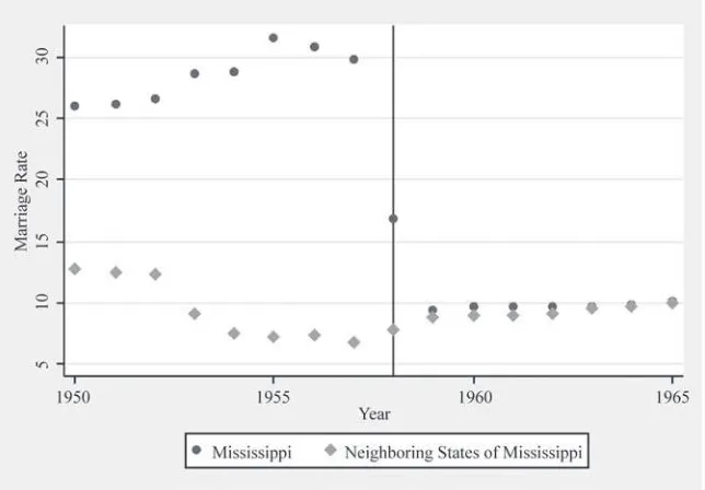
Although the marriage law amendment was passed in 1957, it went into effect in 1958 and immediately resulted in a substantial decline in marriages performed in Mis-sissippi. The resulting decline in Mississippi was a combination of a decline from out–of- state couples and in- state couples who did not meet the requirements. Indeed, Mississippi’s laws prior to 1958 were lenient in comparison to its surrounding states of Alabama, Arkansas, Louisiana, and Tennessee. Figure 2 uses yearly marriage rates from the Vital Statistics to show the decline in Mississippi relative to its surrounding states. Importantly, it shows that, while marriages in Mississippi declined and mar-riages in surrounding states increased, in no way did the increase compensate for the massive decline. Plateris (1966) uses state of residence information from the Missis-sippi State Board of Health to confi rm this (see Appendix Table 1).5 From 1957 to
1959, Plateris (1966) notes, marriages in Mississippi where both spouses resided in the
5. Appendix tables are available at http://prbharadwaj.wordpress.com/papers/. Figure 2
Marriage Rate in Mississippi and Surrounding States
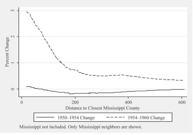
state declined by 20 percent while marriages in Mississippi where both spouses were nonresidents of Mississippi declined by 90 percent. As a result, most of the decline in Mississippi itself was driven by the drop in out- of- state marriages. Out- of- state couples who did not get married in Mississippi could still get married in their home state and many did so. However, even taking the increase in marriages in neighboring states into account, the area in general saw a decline in the number of marriages by 13 percent. I confi rm these fi ndings using county- level marriage data and plotting changes in marriage rates between 1950–54 and 1954–60. Figures 3a and 3b clearly show a large decline after the law change in counties that were closer to the Missis-sippi border (in particular along the MissisMissis-sippi- Alabama border).
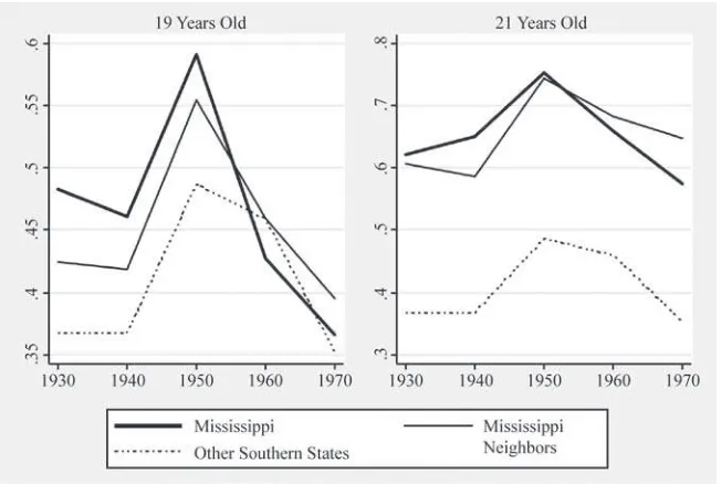
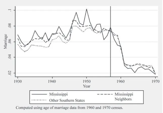
As further evidence, Figure 4a shows the drop in marriages at the state level using census data from 1930 through 1970. This fi gure is also useful in seeing that before 1950 we do not see any Mississippi- specifi c trends in marriages. In fact, between 1930 and 1950, trends in marriage in Mississippi looked very similar to trends in its neighboring states as well as other Southern states.
After 1950, however, we see that the proportion of married 19- year- olds (they were 16–17 when the law was passed) in Mississippi drops sharply below that of all other states. Figure 4b uses age of marriage data from the 1960 and 1970 census to com-pute the fraction of married teenagers. While this fi gure is predictably noisier, the decline in marriage in Mississippi is apparent. Importantly, these graphs show why a difference- in- differences approach is needed. The proportion of married 19- year- olds, or the fraction of married teenagers in other states, also seems to have declined in the late 1950s; hence, it will be crucial to separate the decline due to the secular trend from the decline due to the marriage law.
III. Data and Empirical Strategy
Isolating the impact of the change in marriage law is a critical chal-lenge in this case. It is likely that changes in schooling and fertility of women is caused by local and/or macroconditions unrelated to the change in marriage law. The main strategy used to differentiate the effect of the law from other causes in this paper is a difference- in- differences strategy; however, data limitations for certain outcomes and years determine the type of difference- in- differences strategy used (see Table 1). Critical for my strategy, neighboring states of Mississippi did not experience a change in mar-riage law during this period (1950–60), and no state considered for the analysis expe-rienced a change in compulsory schooling laws. Moreover, Arkansas, Tennessee, and Louisiana’s minimum marriage age for women was 16 while Alabama’s was 14 during 1950–60. In fact, Mississippi was the only state in the country during this decade to have the minimum age at 12 for women—all states had a higher minimum age by 1950.6
One of the main challenges while using a difference- in- differences strategy is to appropriately defi ne treatment and control groups. Section II suggests a few different
T
he
J
ourna
l of H
um
an Re
sourc
es
Table 1
Baseline Comparisons (Means Computed from 1950 and 1954)
Variable
Treatment Control
Difference (Treatment- Control)
Standard Error Mean
Standard
Deviation Mean
Standard Deviation
Panel A - Treatment is Mississippi and neighboring counties, control is remaining counties in neighboring states
Marriages per 1,000 in population 23.09 45.66 10.53 17.96 12.56*** 2.29
Log crude birth rate 3.16 0.22 3.06 0.303 0.09*** 0.022
Percent 14–17- year- olds enrolled 77.64 5.12 76.89 6.14 0.75 0.67
Manufacturing wage 2.78 9.33 4.11 12.77 –1.32 0.95
Percent employed in manufacturing 35.25 27.83 44.33 39.35 –9.08*** 2.909
Farms per 100 in population 0.12 0.04 0.097 0.04 0.02*** 0.002
Percent farms with tractors 27.22 8.56 33.12 13.38 –5.89*** 1.37
Agricultural employment per 1,000 in population 150.93 58.9 115.11 53.92 35.82*** 6.25 Panel B - Excluding Mississippi counties
Marriages per 1,000 in population 19.97 44.7 10.53 17.96 9.44*** 2.44
Log crude birth rate 3.15 0.213 3.06 0.3033 0.088*** 0.027
Percent 14–17- year- olds enrolled 76.02 4.31 76.89 6.14 –0.86 1.23
Bha
ra
dw
aj
621
Percent farms with tractors 27.22 8.56 33.12 13.38 –5.89*** 1.37
Agricultural employment per 1,000 in population 137.85 53.95 115.11 53.92 22.73** 10.7 Panel C - Excluding Mississippi counties and
within 200 miles of Mississippi border
Marriages per 1,000 in population 19.97 44.7 9.56 19.93 10.41*** 3.13
Crude birth rate 3.154 0.213 3.13 0.321 0.022 0.03
Percent 14–17- year- olds enrolled 76.02 4.31 77.53 6 –1.51 1.23
Manufacturing wage 3.73 11.6 4 14.15 –0.269 1.38
Percent employed in manufacturing 36.96 29.17 41.16 33.97 –4.19 3.36
Farms per 100 in population 0.11 0.04 0.09 0.043 0.019*** 0.004
Percent farms with tractors 27.22 8.56 36.44 13.38 –9.216*** 1.59
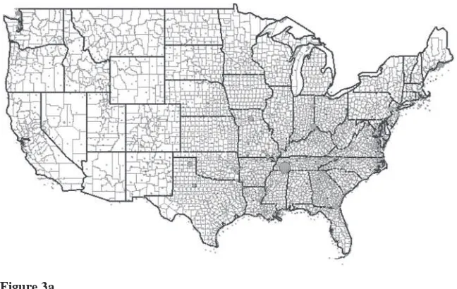
Figure 3b
Change in Marriages 1954–60
Notes: Change in marriages is the percent change from the previous year of available data. Absolute value of the percent change is shown on the maps. County- level data are from the County and City Datebooks 1950, 1954, and 1960.
Figure 3a
ways to defi ne treatment and control groups. The defi nition of treatment is based largely on the degree of data disaggregation available. Using county- level data, we can use distance from the Mississippi border as a continuous measure of treatment or Mississippi and its surrounding counties as treatment and remaining counties in the neighboring states as control as a dichotomous measure of the areas that were affected by the law change (as suggested by Figure 3). Using state- level data, we can use Mississippi and neighboring states as treatment and remaining Southern states (where Southern is defi ned as a census region) as the control, for example. In addition, the nature of the law change implies that younger age groups should be more affected than older age groups. The age dimension of the law changes allows for a triple difference strategy (that is, comparing younger and older age groups across treatment and control states before and after the law change).
However, as I explain below, some of these strategies cannot be used in conjunction due to data limitations. Importantly, some of the data are available for more years, which allows for a more accurate control for trends prior to the law change, another aspect of a difference- in- differences analysis that is quite critical. The subsections below explain in detail the different strategies used.
A. County- Level Analysis
County- level analysis has the distinct advantage that I can examine changes in border counties relative to interior counties of neighboring states. Specifi cally, it allows me
Figure 4a
Proportion of Married Women by Census Year
to construct treatment groups such that the intensity of “treatment” decreases with distance away from the Mississippi border. Comparing counties within the same state that only differ by distance to the Mississippi border reduces the possibility that factors other than the law change in Mississippi are driving the results. However, this strategy comes at the cost of not being able to include Mississippi as part of the results. To include Mississippi as part of the treatment group, I defi ne a more restrictive treatment group comprising counties in Mississippi and counties in neighboring states that share a border with Mississippi. The remaining counties in neighboring states comprise the control group under this specifi cation. Evidence from Section II suggests that this is a reasonable way to assign treatment and control. Under this defi nition of treatment and control, in some specifi cations, I can take advantage of using county- level data by controlling for state- by- year trends.7 A major advantage of count- level data over
census data is that county- level data are available for intercensal years. Marriage rates, for example, are available for the years 1948, 1950, 1954, and 1960 at the county level while fertility is available at the yearly level from 1945–65. This allows me to control accurately for trends prior to the law change.
The disadvantage of using county- level data is that the county- level data do not contain details on sex, race, or age. In particular, data by age would have allowed for
7. Again, doing so would exclude Mississippi counties since all Mississippi counties are defi ned as a “treated” county.
Figure 4b
Fraction of Married Teenagers by Year
sharper analysis because the minimum age and parental consent laws were directed toward younger age groups. In sum, the county- level analysis yields the preferred set of estimates. While using data by age and gender is an important check on the valid-ity of the estimates, the major advantages of using county- level data include using distance from the Mississippi border, as well as data from intercensal years, and being able to control for state- specifi c trends..
The difference- in- differences strategy using county- level data can be estimated as follows:
(1) Outcomeijt = 1Treatijt + 2Postijt + 3(TreatijtXpostijt) + jt + Xijt + ijt
where Outcomeijtstands for an outcome like marriage or enrollment rates in county I in state j at time t.Treatijtdenotes whether the county is defi ned as a “treated” county. In thecase of using distance from the Mississippi border, Treatijtis simply the inverse of distance to theMississippi border. An alternative defi nition of treatment used in this paper is to defi ne all countiesin Mississippi and border counties of neighboring states as treated. In this case, Treatijtis simplya dummy variable, taking the value of 1 for treated counties and 0 for control counties. Postijt is a dummy variable that takes a value of 1 for years after 1957 and is 0 otherwise. The coeffi cientof interest here is three, which is the difference- in- differences coeffi cient. Xijtdenotes a vector of con-trols like tractor use, employment in manufacturing, etc. jt denotes the state- by- year
fi xedeffect, although I can only use this in cases where Mississippi is not included in the analysis. Inthe specifi cations that include Mississippi, I use state and year fi xed effects.8
Due to the inclusion of border counties in neighboring states in the treatment group, standard errors are clustered at the county level. However, results using different lev-els of clusters are shown in the appendix. Bertrand, Dufl o, and Mullainathan (2004) stress the importance of clustering standard errors while using DD techniques to ex-amine the impact of law changes. Because the law was imposed at the state level in Mississippi, an argument could be made that conservativestandard errors are achieved by clustering at the state level. However, clustering at the state level yields fi ve clus-ters in my case leading to large standard errors for some of the results. To deal with a small number of clusters, I use three approaches. First, I use the methodology in Buchmueller, DiNardo, and Valleta (2011) of using “placebo” states to obtain the sam-pling distribution of the difference- in- differences coeffi cient. In other words, Equa-tion 1 is estimated using other states as the treated state and the coeffi cient obtained for Mississippi is compared to the coeffi cient obtained for other states. According to Buchmueller, DiNardo, and Valleta (2011), this procedure results in “conservative and appropriate” standard errors. Second, I can increase the number of clusters under the standard procedure by expanding the control group to counties in Texas, Florida, Oklahoma, Virginia, West Virginia, Georgia, Kentucky, North Carolina, Delaware, and Maryland/Washington D.C. This gives me ten more states to include, increasing the number of clusters to 15. I could also include all states in the country and increase the number of clusters to 50. In general, different clustering procedures do not affect the interpretation of the main results. Even under the most conservative of clustering
8. This specifi cation is:
procedures, most of the results remain statistically signifi cant. Results with different clustering methods are presented in Appendix Table 2.
County- level data for birth rates and enrollment were obtained from the City and County Handbooks for the years 1948, 1950, 1954, and 1960. Data are not available for the intervening years. These data are at the county level and contain important demographic (marriage, fertility, and schooling) and labor market- related variables (wages, tractor use, etc.). The City and County Handbooks get their birth and marriage data from the Vital Statistics. However, not all variables are present for all years, nor are they necessarily in a format that is comparable across years. For example, school enrollment in the City and County Handbook is available for age groups 14–17 in 1950 but only for age groups fi ve to 34 in 1960. Hence, school enrollment data at a comparable level between 1950 and 1960 are obtained from the historical census col-lection from the University of Virginia Library website. The historical census provides county identifi ers, but as it is a census, there are no data on enrollment for any inter-censal year.9 In addition, I obtained yearly county- level births from 1946–65 thanks
to a data collection effort undertaken by Martha Bailey.10
B. State- Level Analysis
Data at the state level come from the census and have the advantage that some of these data contain data by age. Since the law change was intended to affect certain age groups more than others, using age- specifi c information, I can assign treatment status not only by state of residence but also by age. I can do this using census data from 1950 and 1960. Women below the age of 21 (and particularly below the age of 18) in 1957–58 were impacted by the change in marriage law, so women above the age of 21 in 1957 should not be affected by the change in marriage law, or at the very least should be affected less than women below the age of 21. This is because, while proof of age and blood test requirements affected everybody, the age restrictions were an added barrier for women below the age of 21 in 1960. In addition, verifying the results using census data is critical in light of potential misreporting of age in marriage licenses (Blank, Charles, and Sallee 2009). A triple difference- in- differences (essen-tially a state- cohort analysis) exploits the age- specifi c impact of the marriage law.
Using 1950 and 1960 census data at the state level, the estimating equations typi-cally take the following form:
(2) Yijtg = g(Treatijtg * Postijtg * Σg=33 g=14 Aijtg) + 1(Treatijtg * Σg=33 g=14 Aijtg) + 2(Postijtg * Σg=33 g=14 Aijtg) + 3Treatijtg + 4Postijtg
+ 5Σg=33 g=14 Aijtg + υijtg.
Where Yijtgis the relevant outcome (age of marriage, school enrollment, number of children, etc.) for person i in state j at time t belonging to age group g. Treat is a dummy that takes on 1 if the person lives in Mississippi or its neighboring states
9. The historical censuses also do not have marriages and births by sex, race, or age. They simply contain aggregates for the years 1950 and 1960.
and 0 otherwise.11Post is a dummy that is 1 if the year is 1960 and 0 otherwise. A
is a dummy that takes on the value of 1 if the person belongs to age group g and 0 otherwise. The DD estimate is the triple interaction of Age, Treat, and Post, and all lower interaction terms and main effects are included in the regression. Note that the interaction of Treat and Post is not included. The inclusion of all age dummies inter-acted with Treat and Post implies that the double interaction is completely described by this triple interaction.
Triple DD estimates are obtained by comparing the for younger versus older age groups. Standard errors are clustered at the state- year level. The age groups (as of 1957) are 11–14, 16–20, 21–25, and 26–30. These groupings were made to facilitate presentation of the results and to clearly show that the main impacts of the marriage law are coming through younger age groups.12 Although the triple interaction for all
age groups is included, double interactions and main effects for age group 26–30 form the excluded group. A key advantage of the census data is that in 1960 the census asked about age at fi rst marriage for the sample that reports having been married. (In 1950, while they do not ask about age at fi rst marriage, they ask about duration of mar-riage, from which we can impute the age of marriage for those who report currently being married.) Age of marriage in the census is likely to be more reliable than age of marriage in the Vital Statistics because the Vital Statistics records age of marriage at the time of marriage when incentives to misreport age might be higher. In the census, there are no such incentives to misreport.
The disadvantage of using census- level data is that there are no data for the inter-censal years. This limits the extent to which I can control for differential trends in the 1950s. Moreover, it is diffi cult to accurately assign treatment status with just state- level identifi ers. Because border counties of neighboring states of Mississippi were also affected, I present results using two versions of a treatment group. My preferred estimate comes from using just Mississippi and its neighboring states as the treat-ment group and the remaining states in the southern region (as defi ned by the census) as the control group. As a robustness check, I assign only Mississippi as the treatment group and treat its neighbors as the control group.
As a compromise between the county- level data and the census data, I collected data from the Vital Statistics at the state level for outcomes such as births and il-legitimate births. The state- level Vital Statistics were available from 1952 onward and provide yearly information on births and illegitimate births by age and race of the mother. Although I cannot conduct a distance- level analysis with this data, I can esti-mate Equation 1 using Mississippi as the treated state and its neighbors as the control states for various age groups.
11. State of residence from the census is used to assign persons to treatment or control group. Because the law change was implemented in 1958, only two years passed between the passage of the law and the 1960 census. In 1960, 9 percent reported having lived in a different state in the last fi ve years in the treatment group and 12 percent in the control group. Moreover, the migration rates are much lower for blacks than for whites. Only 3 percent of blacks in the treatment group in 1960 report having lived in a different state in the past fi ve years while the same statistic for the control group is around 5 percent. The 1950 census does not have comparable migration information.
IV. Results
This section presents results from estimating Equations 1 and 2. Be-cause county- level estimates are the preferred estimates, for each outcome I fi rst pres-ent county- level estimates followed by state- level estimates.
A. Marriage Decline
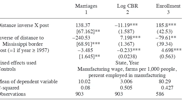
While Figures 1–4 largely establish the impact of the law change on marriage rates, this section provides more specifi c evidence. Using distance to the Mississippi border as the defi nition of treatment, Table 2 estimates Equation 1 and shows that distance to border matters for marriage rates after 1957 (the interaction of distance inverse and post dummy) and that this is a statistically signifi cant effect. In order the make the table interpretable, I use the inverse of distance to Mississippi border; therefore, the interaction term suggests that places close to the Mississippi border experienced an increase in marriages after the law change. This confi rms the casual observation in Plateris (1966, replicated in Appendix Table 1) as well as Figure 5. Note that this increase does not make up for the overall decrease in number of marriages.
The downside to this defi nition of treatment is that it necessarily excludes Missis-sippi from the analysis. In order to include MissisMissis-sippi as a treated group, I defi ne
Mis-Table 2
Impact of Marriage Law and Distance from Mississippi Border
Marriages
Distance inverse X post 138.37 –11.19*** 185.8***
[67.162]** (1.587) (42.53)
Controls Manufacturing wage, farms per 1,000 people,
percent employed in manufacturing
Mean of dependent variable 10.02 3.006 80.29
R- squared 0.08 0.505 0.427
Observations 903 903 586
Notes: Marriages are marriages per 1,000 in population, births are log births per 1,000 in population, and enrollment is the percentage of 14–17- year- olds enrolled in school. Distance (in miles) is computed using latitude- longitude information on counties and distance to the closest Mississippi county is computed using the Haversine formula. Mississippi is excluded from these regressions, as all points within Mississippi have a distance of 0. Counties from neighboring states of Mississippi used.
sissippi and bordering counties as the treatment group with remaining counties in the neighboring states as the control group. Table 3 shows estimates of Equation 1 with various controls. Although the treatment group defi nition stays the same (Mississippi and counties in Alabama, Arkansas, Tennessee, and Louisiana that border it), Column 1 uses all southern counties as the control group. Column 2 shows that restricting the control group to counties in the neighboring states of Mississippi does not change the results much. In Column 3, I add state and year controls, which again do not make any difference (I can use state fi xed effects, as the treatment group consists of coun-ties within states). Columns 4 and 5 add county- level controls like manufacturing wages, employment in manufacturing industries, number of farms, and employment in agriculture—these are key labor market- related variables, and trends in these vari-ables could affect marriage rates independently of the change in law. Since agricultural employment was only collected for 1950 and 1960, Column 5 has fewer observa-tions than Column 4. Comparing coeffi cients across Columns 1–5 shows that adding controls does not change the coeffi cient on the difference- in- differences estimator (the interaction of Treatment and Post dummies). The results indicate that after the change in law, treatment counties experienced a drop of ten marriages per 1,000 in the population. Prior to 1957, the rate of marriages per 1,000 in Mississippi and its
Figure 5
Percent Change in Number of Marriages
Table 3
Impact of Marriage Law on Marriages
Marriages Per 1,000 in Population
All Treatment Counties Used Mississippi Not Included
1 2 3 4 5 6 7
Post X treatment –12.678 –12.509 –12.509 –13.389 –10.414 4.96 4.303
[3.656]*** [3.749]*** [3.756]*** [4.027]*** [4.077]** [1.241]*** [0.910]*** Treatment (=1 if Mississippi
or county bordering Mississippi)
11.657 11.626 –1.232 0.628 1.83 –5.6 –5.309
[4.010]*** [4.104]*** [1.319] [1.501] [2.509] [0.808]*** [0.737]***
Post (=1 if year ≥ 1957) –0.135 –0.305 –0.026 –2.188 –4.195 –2.662 2.902
[0.451] [0.919] [1.093] [1.451] [1.748]** [1.413]* [0.790]***
Manufacturing wage –0.051 –0.042 –0.037 –0.051
[0.039] [0.032] [0.032] [0.033]
Farms per 1,000 in population 1.186 20.608 11.794 1.978
[21.637] [29.631] [17.796] [17.846]
Percent employed in manufacturing 0.047 0.005 0.048 0.044
[0.040] [0.029] [0.043] [0.043]
Percent employed in agriculture –0.037
631 in southern
U.S.A.
Mean of dependent variable 12.04 13.05 12.82 12.98 10.05
R- squared 0.01 0.04 0.09 0.09 0.08 0.08 0.16
Observations 5,807 1,532 1,532 1,149 766 903 903
Notes: Columns 1–5 use a state- year cluster, and Columns 6 and 7 use a treatment group, state- year cluster since Mississippi is excluded in these regressions. Dependent variable is marriages per 1,000 of the population. Data from city and county data book for years 1948, 1950, 1954, and 1960 are used. Population at the county level for 1950 and 1960 is used to compute the percentages (1954 numbers are divided by the population in 1950). Treatment is 1 if state is Mississippi and border counties. Percent employed in manufacturing and agriculture also uses population from 1950 and 1960 as the base. Agricultural employment data are only available for 1950 and 1960. Manufacturing employment and wages data are not available for 1948. Regression follows Equation 1 in the paper.
neighboring counties was around 22 (Table 1). Table 2 shows a remarkable decline of almost 50 percent compared to the prelaw change average.
Columns 6 and 7 show the impact of the marriage law when we exclude Mississippi from the analysis. Because the entire state of Mississippi is part of the treatment group, when I include state- by- year fi xed effects, only the border counties in the neighboring states are identifi ed. Hence, the DD estimator has a positive sign for these columns. Comparing Columns 6 and 7 also shows that adding state- by- year fi xed effects, which control for state- specifi c trends, does not change the fact that marriage rates were af-fected by the change in law. This suggests that the DD estimator is indeed picking up the change in marriages due to the change in law as opposed to changes due to other differential trends at the state level.
Moving to state- level analysis using the data from the census, Table 4 shows that for younger age groups among women, the probability of being married (this is
de-fi ned throughout this analysis as being married by the time of the relevant census) decreased and the age of marriage increased by 1960. This table is created by esti-mating Equation 2 using fi ve- year age groups instead of individual age dummies for easy interpretation. The omitted age group is the age group 31–35. Compared to this age group, Column 6 in Table 2 shows, for example, that black women in the age group 16–20 as of 1957 experienced an increase in marriage age of nearly 0.4 years. Compared to the average age of marriage for black women in the sample (19 years), the increase in marriage age is quite large. The same applies for the probability of being married. Black women in the age range 16–20 are thirteen percentage points less likely to report being married by 1960, representing a 23 percent change from the mean probability of being married.
Comparing the difference- in- differences coeffi cient across various age groups, it is clear that the most impacted age group is the group aged 16–20 in 1957–58 rather than, say, the age group of 26–30. This is reassuring as the changes in the marriage law were mainly directed at younger age groups due to various age restrictions.
Results using census data show that most of the overall effects appear to be driven by blacks. Blacks formed a large portion of the overall population in the South—by 1960, blacks were about 26 percent of the population in Mississippi and its surround-ing states (Mississippi’s population at the time was nearly 51 percent black). More-over, among black women, the effect on marriages extends to the 21–25 age group as well. This is likely due to restrictions like proof of age and blood tests being a greater burden on blacks than on whites during this time period. This is similar to Buckles, Guldi, and Price (2009), who fi nd that blood test laws for marriages were more of a deterrent to blacks. Thus, relative to whites, it appears that the marriage law changes in Mississippi raised the cost of marriage mainly for blacks.
B. Fertility
Bha
11–15 –0.013 –0.007 –0.027 –0.21 –0.017 –0.126 –0.006 –0.007
[0.014] [0.003]* [0.092] [0.273] [0.024] [0.234] [0.014] [0.111]
16–20 –0.057 –0.042 0.154 –0.103 –0.139 0.39 –0.021 0.09
[0.023]** [0.023]* [0.101] [0.107] [0.043]*** [0.159]** [0.025] [0.123]
21–25 –0.014 –0.015 –0.069 0.061 –0.073 –0.195 0.009 –0.013
[0.015] [0.014] [0.152] [0.144] [0.035]** [0.491] [0.015] [0.242]
26–30 –0.011 0.013 0.094 –0.055 –0.009 –0.245 –0.007 0.311
[0.010] [0.013] [0.285] [0.178] [0.023] [0.451] [0.010] [0.320]
Mean of dependent variable
0.614 0.457 18.99 21.29 0.551 19.13 0.633 18.95
R- squared 0.46 0.48 0.17 0.21 0.42 0.18 0.47 0.17
Observations 175,045 168,111 58,763 43,851 39,867 10,302 134,610 48,265
Notes: Data from IPUMS 1 percent sample from years 1950 and 1960. All regressions are weighted by census person weights. Probability of marriage is a variable that is 1 if married, 0 otherwise at the time of the Census. Age of marriage is conditional on marriage. Regressions refl ect estimation of Equation 2 in the paper. Controls included are all main effects of age groups and treatment group status.
log crude birth rate as the dependent variable.) However, unlike the graphs and fi gures used to show the decline in marriages, the drop in births is smaller in magnitude and, hence, is better represented in regression tables. Figure 6 shows that areas close to the border after the law change show greater negative changes (this was not the case before the law change) than areas further away.
Table 5 follows a similar estimation strategy as Table 3. Equation 1 is estimated using log of births per 1,000 in the population as the dependent variable. Once again, it is clear that adding controls does not change the coeffi cients. Although Table 3 shows that marriages increased slightly in the border counties, Table 4 shows that births decreased (Columns 6 and 7). This is not inconsistent at all, as the overall mar-riages in the border counties did decline. It is just that before the change in law, all the marriages were being recorded in Mississippi. The coeffi cients across the main specifi cations including Mississippi suggest a drop of around 5–6 percent. This drop in births is quite substantial considering that between 1910 and 1954 the drop in crude birth rate was around 16 percent for the entire country.
Tables 6a and 6b estimate Equation 1 using yearly county- level data. I choose to present this separately and not as my main specifi cation as I do not have data for control variables like wages and employment at the yearly level. Table 6a uses these
Figure 6
Percent Change in Number of Live Births
yearly data and defi nes years after 1957 as years affected by the law change. The difference- in- differences coeffi cient in this table is negative throughout, even with the inclusion of state and state- by- year fi xed effects. The results also seem robust to the inclusion of state linear and state nonlinear time trends (the coeffi cients of interest are just shy of signifi cance at the 10 percent level in the fi rst panel of Table 6a). The middle panel of 6a estimates the same relationships but restricts the control group to counties within 200 miles of the Mississippi border. These counties are arguably more similar to Mississippi (see Table 1) prior to the law change. Again, the results are largely consistent with the top panel. These results are not affected by the years chosen to be in the sample. In the bottom panel of this table, I restrict attention to the years 1955–60, and the effects are largely unchanged, suggesting that the effects are not driven by earlier or later time periods. An important way these results differ from the results in Table 5 is in the magnitude of the coeffi cients. The coeffi cients in Table 6a are quite a bit smaller than those in Table 5. One reason for this is the likely changes in 1954–60 not related to the marriage law change; hence, Table 5 might be playing up some of these larger reasons behind the fertility decline. The estimates in Table 6a suggest a decline in fertility of around 2 percent.
The other major advantage of the yearly data is that I can estimate a difference- in- differences estimate using each year from 1950–63 as a placebo year in which the law change occurred. In other words, I can treat each year as though it were a “treated” year and compute the difference- in- differences estimates. Hence, if events in 1956 Mississippi unrelated to the law change were driving the fertility results, the difference- in- differences coeffi cient for that year should be negative and signifi cant. Table 6b shows that it is precisely in 1958 that the difference- in- differences
coef-fi cient becomes negative and statistically signifi cant. 13 In the years prior to 1958, the
difference- in- differences coeffi cient is positive (although not statistically signifi cant), indicating that the treated counties had a higher birth rate compared to the control counties, and this begins to change precisely in 1958. However, as is clear from the estimates, while consistent with the idea that the law change is driving these results, the existence of a mild pretrend (although not statistically signifi cant) and the lack of a strict trend- break around 1957 in some specifi cations, should be treated with caution. Accounting for state- specifi c trends does not change the results much, ex-cept that some of the difference- in- differences coeffi cients are no longer statistically signifi cant.
Another source of yearly data on fertility is the Vital Statistics tabulations of the number of births at the state level. One advantage of these tabulations over the yearly county- level data is that these tabulations are available by race and age. Tables 7a and 7b explore the fraction of births by race and age in a similar difference- in- differences setup as in Equation 1. Table 7a shows that the decline in births is among younger age groups and is larger in magnitude for blacks. Hence, it corroborates the results presented earlier showing that the law perhaps affected blacks more. The Vital Statistics also reports the number of illegitimate births by age and race for this time period. For younger women, I fi nd an increase in illegitimate births after the passage of the law (Table 7b). Hence, while the law in effect prevented younger age groups
Table 5
Impact of Marriage Law on Crude Birth Rate
Log Births per 1,000 in Population
All Treatment Counties Used Mississippi Not Included
1 2 3 4 5 6 7
Post X treatment –0.0158 –0.0424* –0.0424* –0.0584*** –0.0558** –0.136*** –0.113***
(0.0185) (0.0216) (0.0216) (0.0218) (0.0274) (0.0286) (0.0307)
Treatment (=1 if Mississippi or county bordering Mississippi)
0.0781*** 0.0903*** 0.0487 0.0769** 0.0575* 0.104*** 0.0952***
(0.0213) (0.0253) (0.0397) (0.0308) (0.0324) (0.0338) (0.0358)
Post (=1 if year ≥ 1957) –0.269*** –0.242*** –0.310*** –0.320*** –0.300*** –0.322*** –0.371***
(0.00609) (0.0126) (0.0144) (0.0168) (0.0185) (0.0182) (0.0221)
Manufacturing wage –0.00117** –0.00139*** –0.00142*** –0.00130***
(0.000479) (0.000497) (0.000463) (0.000461)
Farms per 1,000 in population –3.222*** –4.138*** –3.336*** –3.353***
637 Percent employed in
agriculture
0.000953*** (0.000359)
Fixed effects used None None State, Year State, Year State, Year State, Year State X Year
Control group All counties
in southern U.S.A.
Counties in states neighboring Mississippi only
Observations 4,650 1,372 1,372 1,029 686 810 810
R- squared 0.139 0.182 0.371 0.501 0.503 0.514 0.541
Notes: Dependent variable is log births per 1,000 of the population. Data from city and county data book for years 1948, 1950, 1954, and 1960 are used. Population at the county level for 1950 and 1960 is used to compute the percentages (1954 numbers are divided by the average population between 1950 and 1960). Treatment is 1 if state is Mississippi and border counties. Agricultural employment data are only available for 1950 and 1960. Manufacturing employment and wages data are not available for 1948. Regressions refl ect estimation of Equation 1 in the paper. Outliers in the dependent variable (top and bottom 5 percent of the counties with changes in birth rates) removed. Including these counties increases the magnitude of the effect to around 8–9 percent in Columns 1–5 and the effects remaining statistically signifi cant. These estimates are presented in Appendix Table 13.
T
he
J
ourna
l of H
um
an Re
sourc
es
Table 6a
Log Birth Rates Per 1,000 of Female Population
1 2 3 4 5
Full sample 1950–63
Difference- in- difference –0.0179** –0.0179** –0.016 –0.0159 –0.00828
(0.00850) (0.00851) (0.01) (0.0100) (0.0135)
Dummy for post (year > 1957) 0.00643 0.0218*** 0.0164** 0.0241*** 0.0108
(0.00529) (0.00707) (0.00656) (0.00595) (0.0135)
Dummy for treatment group 0.174*** 0.0924** 0.0916** 0.0916** 0.0883**
(0.0200) (0.0361) (0.0365) (0.0365) (0.0374)
Other controls None State & Year FE State linear
time trends
State quadratic time trends
State X Year FE
Mean of dependent variable 4.791 4.744
Observations 5,362 5,362 5,362 5,362 4,214
R- squared 0.130 0.313 0.314 0.315 0.303
Full sample 1950–63, within 200 miles of Mississippi
Difference–in- difference –0.0240** –0.0240** –0.0204* –0.0204* –0.0183
(0.00938) (0.00940) (0.0114) (0.0114) (0.0149)
Dummy for post (year > 1957) 0.0126* 0.0401*** 0.0186** 0.0315*** –0.0757***
(0.00660) (0.00858) (0.00847) (0.00794) (0.0185)
Dummy for treatment group 0.119*** 0.0709** 0.0694* 0.0693* 0.0684*
Bha
ra
dw
aj
639
Mean of dependent variable 4.848 4.814
Observations 3,556 3,556 3,556 3,556 2,408
R- squared 0.071 0.223 0.219 0.222 0.251
Restricted to 1955–60
Difference–in- difference –0.0218*** –0.0218*** –0.0102 –0.0102 –0.0195
(0.00782) (0.00783) (0.00987) (0.00987) (0.0124)
Dummy for post (year > 1957) 0.0149*** 0.0185*** –0.0168** –0.0168** 0.00424
(0.00513) (0.00684) (0.00702) (0.00702) (0.0102)
Dummy for treatment group 0.181*** 0.0924** 0.0866** 0.0866** 0.0913**
(0.0219) (0.0389) (0.0399) (0.0399) (0.0408)
Other controls None State & Year FE State linear
time trends
State quadratic time trends
State X Year FE
Mean of dependent variable 4.795 4.759
Observations 2,298 2,298 2,298 2,298 1,806
R- squared 0.128 0.337 0.340 0.340 0.330
Notes: Data used are country level log fertility rates per 1,000 of the female population. Treatment group is all of Mississippi and counties in neighboring states sharing a border with Mississippi. Control groups are all other counties in neighboring states of Mississippi. Since all of Mississippi is considered part of the treatment group, regressions that use StateXYear fi xed effects drop Mississippi and only use border counties as the treatment group. Regressions refl ect estimation of Equation 1 in the paper.
Robust standard errors in brackets.
Table 6b
Log Birth Rates Per 1,000 of Female Population
Difference-
Controls State, Year FE StateXYear FE State, Year FE StateXYear FE
Observations 5,362 4,214 3,556 2,408
Notes: Reported coeffi cients are difference- in- difference coeffi cients for each year. Separate regressions are estimated for each coeffi cient in a specifi cation similar to Equation 1. Treatment and control group defi nitions are the same as in Table 5. Columns including StateXYear FEs have fewer observations as Mississippi is omitted from those regressions (as all of Mississippi is treated as opposed to just border counties in neighbor-ing states).
Robust standard errors in brackets.
from marrying and having children, it did have some unintended consequences as it raised the number of illegitimate children.
Data from the census reveal that women affected by the law change in Mississippi were less likely to have children compared to women not affected by the law change. Table 8 shows that, compared to older groups in control counties, black women in the age group 16–20 are nearly ten percentage points less likely to have a child. The fraction of black women in 1950 in this age range that had children was around 43 per-cent. Hence, relative to that mean, this is a large effect. Comparing the DD coeffi cient of this age group to the age group 26–30 shows that it was the younger groups that were most affected. As in the case of marriage rates, blacks appear more affected than
Table 7a
Impact of Marriage Law on Births by Age of Mother
Percent of Total Births by Age of Mother
Under 15
Post (=1 if year > 1957) 0.066 0.301 –0.683
[0.030]* [0.336] [0.336]*
Post (=1 if year > 1957) 0.04 2.331 1.646
[0.014]** [0.222]*** [0.219]***
Mean of dependent variable
R- squared 0.68 0.96 0.94
Observations 129 129 129
Notes: Dependent variable is percent of total births that are born to mothers of the relevant age group. Data are from the Vital Statistics, for years 1952–64. Treatment group is Mississippi, Alabama, Louisiana, and Tennessee. Arkansas did not report statistics for this variable during this period. The control group consists of Florida, North Carolina, Kentucky, Virginia, West Virginia, and Texas. Georgia, Delaware, and the District of Columbia did not consistently report this variable for these years. Regressions refl ect estimation of Equation 1 in the paper. Only controls used are state and year fi xed effects.
whites and seem to be driving the overall results. This is perhaps another reason why the results in the overall county- level data sets are perhaps a bit muted in comparison. County- level data by race might show sharper decreases.
Taken together, the results from county- and state- level data support the idea that increasing barriers to marriage led to a decrease in birth rates, at least in the immediate short run, by the early 1960s. Later in this section, I examine some of the long- run consequences on fertility due to the change in marriage law in Mississippi. However, given the larger declines in fertility that were taking place all over the country during this period, some of the declines using broader differences (1954–60, or 1950–60) could be capturing more than just the changes due to the law change. However, the results by distance to the Mississippi border, analysis by age of the mother, and the
Table 7b
Impact of Marriage Law on Illegitimate Births
Percent Illegitimate (of Total)
Post (=1 if year > 1957) –12.332 0.952 –1.384
[1.455]*** [0.777] [0.704]*
Post (=1 if year > 1957) –5.74 –1.848 –1.044
[3.642] [0.291]*** [0.080]***
R- squared 0.35 0.78 0.88
Observations 129 130 130
Notes: Dependent variable is percent of total births that are illegitimate to mothers of the relevant age group. Data are from U.S. Vital Statistics for years 1952–64. Treatment group is Mississippi, Alabama, Louisiana, and Tennessee. Arkansas did not report statistics for this variable during this period. The control group con-sists of Florida, North Carolina, Kentucky, Virginia, West Virginia, and Texas. Georgia, Delaware, and the District of Columbia did not consistently report this variable for these years. Regressions refl ect estimation of Equation 1 in the paper. State and year fi xed effects are the only controls.
Bha
ra
dw
aj
643
Overall Blacks Whites
Difference- in- Difference Coeffi cient, Age in 1957
Number of Children
1
Probability of One Child
2
Number of Children
3
Probability of One Child
4
Number of Children
5
Probability of One Child
6
11–15 –0.006 –0.004 –0.024 –0.016 0.007 0.006
[0.012] [0.008] [0.022] [0.013] [0.008] [0.006]
16–20 –0.088 –0.04 –0.215 –0.091 –0.044 –0.019
[0.054] [0.025] [0.079]** [0.030]*** [0.058] [0.032]
21–25 –0.052 –0.028 –0.089 –0.083 –0.068 –0.021
[0.101] [0.022] [0.170] [0.035]** [0.092] [0.022]
26–30 –0.018 –0.006 0.366 0.037 –0.162 –0.025
[0.140] [0.017] [0.245] [0.031] [0.113] [0.017]
Mean of dependent variable 1.199 0.490 1.291 0.422 1.171 0.510
R- squared 0.29 0.33 0.24 0.24 0.32 0.36
Observations 175,045 175,045 39,867 39,867 134,610 134,610
Notes: Data from IPUMS 1 percent sample from years 1950 and 1960. All regressions are weighted by census person weights. Number of children is the variable “nchild” from the census. Using “chborn” does not change the results. Regressions refl ect estimation of Equation 2 in the paper. Controls included are all main effects of age groups and treatment group status.
results using county- level yearly data should mitigate concerns that forces other than the marriage law are driving all the results.
C. School Enrollment
Goldin and Katz (2002) fi nd that when women have control over their fertility, they invest more in their career. Does a change in marriage law discouraging early marriage have a similar effect? According to Field and Ambrus (2006), a mandated increase in the minimum age of marriage should result in greater educational attainment for women. Using the same empirical strategies as before, I examine whether the change in law led to greater educational attainment and enrollment. Unfortunately, data on school enrollment are not as extensive for this period as the data on fertility. For ex-ample, there are no comparable yearly county- or state- level data on enrollment rates for all treatment and control areas.
The county- level data for enrollment only exist for 1950 and 1960 (this is because comparable enrollment data were only available via the historical census). Hence, I cannot produce a graph similar to Figures 5 and 6; instead, in Figure 7, I plot the 1960–50 difference against distance to the Mississippi border. The graph indicates a
Figure 7
Difference in Percentage of 14–17- Year- Olds Enrolled in School
strong trend similar to Figure 5, in that areas close to the border experience the high-est gains in enrollment. Column 3 in Table 2 shows that counties closer to the border after 1957 had statistically higher enrollment rate gains compared to counties fur-ther away (the estimations follow Equation 1 using enrollment rates as the dependent variable).
Table 9 shows estimates of the DD coeffi cients for school enrollment. Similar to Tables 3 and 5, I estimate Equation 1 using percentage of 14–17- year- olds enrolled in school as the dependent variable. The DD estimates across all specifi cations are robust to the addition of controls and suggest that the change in marriage law led to a 2.5 percentage point increase in school enrollment for this age group. Because overall school enrollment rates were quite high, this represents a small increase of 3 percent over the mean enrollment at that time. During the decade of 1950–60, there were no changes to compulsory schooling laws in Mississippi or its neighboring states (Dahl 2009). These fi ndings are in line with Field and Ambrus (2006), who posit that a compulsory increase in marriage age will lead to greater school attainment. Unfor-tunately, the county- level data do not permit an analysis of schooling attainment by 1960 because schooling attainment data are only collected for people who are too old to be affected by the law.
Using data from the census, I show that black enrollment rates for the younger age groups were the most impacted. Compared to older age groups and to the control states, Table 10 shows that black men and women between ages 16–20 had higher enrollment rates in 1960. As in the case of the other outcomes already examined, the overall results appear to be driven by the results for blacks. A concern might be that these results are driven by changes in the quality of education during this period in treatment compared to control groups. In Appendix Figures 1 and 2, I show that treat-ment groups did not have a differential change in conventional school quality mea-sures during this time period. Moreover, Appendix Table 7a shows that employment and wages did not change differentially in treatment areas during this time period, thus making it unlikely that changes in returns to education explain the increase in enrollment rates. (I explain Appendix Table 7a in detail in the section on robustness checks.)
D. Evidence From Law Changes in Other States
In 1957, a few other states (not those in our treatment or control group) also instituted changes in their marriage laws. These changes, however, did not alter the minimum age of marriage but instead increased premarital requirements as in the case of South Carolina, where a parental affi davit was required for parties younger than 16. Other states more broadly instituted requirements for blood tests (some of these were re-pealed in the 1980s as discussed in Buckles, Guldi, and Price 2011). The states that experienced a change in law around the same time period were Arizona, New Mexico, Iowa, Indiana, and South Carolina (Plateris 1966).14 Using the same strategy as in
Table 9
Impact of Marriage Law on School Enrollment
Percent of 14–17- Year- Olds Enrolled in School
All Treatment Counties Used Mississippi Not Included
1 2 3 4 5 6 7
Post X treatment 2.65 2.658 2.658 2.547 2.244 2.857 2.075
[0.501]*** [0.573]*** [0.575]*** [0.599]*** [0.615]*** [1.121]** [0.943]** Treatment (=1 if Mississippi or
county bordering Mississippi)
2.029 0.745 –1.608 –1.34 –0.656 –1.485 –1.073
[0.549]*** [0.620] [0.858]* [0.801]* [0.755] [0.977] [0.933]
Post (=1 if year ≥ 1957) 6.725 6.694 6.694 5.985 4.735 5.941 6.825
[0.225]*** [0.357]*** [0.358]*** [0.430]*** [0.450]*** [0.457]*** [0.668]***
Manufacturing wage 0.027 0.03 0.03 0.03
[0.013]** [0.014]** [0.014]** [0.015]**
Farms per 1,000 in population –10.799 30.404 –11.361 –7.806
[7.630] [11.814]** [9.276] [9.340] Percent employed in
manufacturing
0.024 0.011 0.026 0.031
[0.008]*** [0.007] [0.009]*** [0.009]*** Percent employed in
agriculture
647 in southern
U.S.A.
Mean of dependent variable 79.04 80.85 80.3
R- squared 0.2 0.31 0.42 0.45 0.48 0.42 0.45
Observations 2,476 750 750 750 750 586 586
Notes: Dependent variable is percent of 14–17- year- olds who are currently enrolled in school. Data from the historical census of 1950 and 1960 are used. Treatment is 1 if state is Mississippi and border counties. Percent employed in manufacturing and agriculture uses population from 1950 and 1960 as the base. Agricultural employment data are only available for 1950 and 1960. Regressions refl ect estimation of Equation 1 in the paper.
Table 10
Impact of Marriage Law Using Census Data
Difference- in- Difference
11–15 0.022 –0.01 0.219 0.242 0.019 –0.116 0.02 0.274
[0.023] [0.029] [0.166] [0.171] [0.048] [0.290] [0.026] [0.165]
16–20 0.043 –0.004 0.388 0.327 0.097 0.053 0.024 0.397
[0.015]*** [0.026] [0.184]** [0.344] [0.037]** [0.360] [0.021] [0.255]
21–25 0.012 0.019 –0.027 0.248 0.011 –0.004 0.011 0.006
[0.010] [0.013] [0.194] [0.268] [0.016] [0.495] [0.013] [0.248]
26–30 –0.008 –0.013 –0.093 0.008 0.005 –0.499 –0.013 0.14
[0.016] [0.033] [0.194] [0.223] [0.031] [0.521] [0.016] [0.274]
Mean of dependent variable 0.271 0.326 7.176 7.119 0.287 5.785 0.266 7.589
R- squared 0.49 0.39 0.49 0.46 0.46 0.53 0.5 0.48
Observations 92,666 90,218 175,045 168,111 18,552 39,867 73,796 134,610
Notes: Data from IPUMS 1 percent sample from years 1950 and 1960. All regressions are weighted by census person weights. Regressions refl ect estimation of Equation 2 in the paper. Controls included are all main effects of age groups and treatment group status.
Equation 2 and using census data, we can examine whether these changes in law resulted in decreases in marriage rates and fertility.
Table 11 suggests that marriage laws had little impact in Arizona, New Mexico (I combine these states into one treatment group since they share a border), and Indiana on the probability of marriage for different age groups. However, in Iowa there does appear to be a sizable effect concentrated in the early age groups, just as in Missis-sippi. However, Mississippi had an equally sizable negative effect for the next age category as well (this coeffi cient is just shy of signifi cance at the 10 percent level). Note that the results for Mississippi are different in this table as I use a more restricted version of treatment and control (Mississippi is treatment and neighboring states are control). This is to make it compatible with the other states examined, where I use just the state as the treated area and its neighbors as the control. Comparing the results of other states to that of Mississippi shows that the law changes in Mississippi had a much bigger impact than elsewhere. This is likely due to the age and other restrictions included in the new Mississippi law; these were not features of the law changes in other states, which focused mainly on blood tests. It is also likely that, because blacks were more impacted by the law change (blood tests and other requirements were likely more expensive for blacks) and blacks comprised a signifi cant fraction of the popula-tion in Mississippi, we see larger effects in Mississippi.
E. Long- Run Outcomes
Using the census of 1970 and 1990, I examine the long- run impacts of the law change. I do this by using age in 1957 as a variable that defi nes treatment, along with residence in Mississippi and neighboring states. For example, I consider a 17- year- old living in Mississippi in 1957 as treated and a 30- year- old in Mississippi in 1957 as untreated. The difference- in- differences comes from using other states in the southern United States as my control states. Moreover, I examine all long- run outcomes only for black females since they are the most affected group. The short- run effects for whites are quite muted, so the long effects are equally negligible.
Appendix Table 5 shows that people affected by the law in the relevant states had, by 1970, a higher age at marriage and fewer children. However, there is no impact on the probability of marriage or the probability of having a child. Hence, these results are very consistent with the notion that marriage laws affect the timing of marriage and fertility but not the extensive margin of these decisions themselves. There appears to be a positive effect on high school completion although this effect is not signifi cant. Panel B of Appendix Table 5 conducts a placebo test to ensure that the long- run results are not picking some inherent trend in reporting by 1970. Using age groups that were not affected by law, I fi nd no evidence of similar results for the placebo group. Indeed, the few results that are signifi cant go in the opposite direction.
T
he
J
ourna
l of H
um
an Re
sourc
es
Table 11
Impact of Marriage Law Using Census Data
Difference- in- Difference Coeffi cient, Age in 1957
Probability of Marriage: Women
Mississippi 1
Arizona and New Mexico 2
Indiana 3
South Carolina 4
Iowa 5
11–15 –0.0362** 0.00273 –0.0106 0.00733 –0.0249*
(0.0179) (0.0202) (0.0118) (0.0163) (0.0136)
16–20 –0.0395 –0.0274 –0.0161 –0.0269 –0.0121
(0.0262) (0.0274) (0.0199) (0.0267) (0.0261)
21–25 –0.0189 0.0136 0.0330*** 0.00647 –0.0190
(0.0184) (0.0189) (0.0122) (0.0184) (0.0160)
26–30 –0.00322 –0.0208 –0.0260*** 0.0131 –0.0121
(0.0141) (0.0151) (0.00937) (0.0164) (0.0136)
Mean of dependent variable 0.604 0.649 0.611 0.591 0.600
Observations 49,517 83,779 104,196 39,553 65,760
Notes: Data from IPUMS 1 percent sample from years 1950 and 1960. Regressions represent estimation of Equation 2 in the paper. For each state in the columns, the neigh-boring states are used as a control group. Please see appendix for list of control states used for each treated state. Controls included are all main effects of age groups and treatment group status.