Market Basket Analysis
in Retail
Gerard Reig Grau
May 2017
Advisor: Miquel Sànchez-Marrè
Dept. of Computer Science (UPC)
MASTER IN ARTIFICIAL INTELLIGENCE
FACULTAT D’INFORMÀTICA DE BARCELONA (FIB)
FACULTAT DE MATEMÀTIQUES (FM)
ESCOLA TÈCNICA SUPERIOR D’ENGINYERIA (ETSE)
UNIVERSITAT POLITÈCNICA DE CATALUNYA (UPC) – BarcelonaTech
UNIVERSITAT DE BARCELONA (UB)
Abstract
This Master Thesis memory describes a full end-to-end data science project performed in CleverData, a successful start-up specialized in data mining techniques and analytics tools. This project was performed for one of its clients, which is an important retail company from Spain. The aim of the project was both the analysis of the possibly different selling behaviour of the stores or shops of the client and the analysis of customers’ purchase behaviour, also known as Market Basket Analysis, to confirm the hypotheses from the client regarding the existence of different customer purchasing profiles and different store selling profiles in its company. The project was divided in three tasks.
The first one was oriented to the study, detection and validation of different behaviour profiles of the shops/stores of the client. This analysis was done by means of a descriptive process using clustering techniques. In order to guarantee a minimum robustness of the profiles obtained, three clustering algorithms were used: a hierarchical agglomerative clustering technique, a partitional clustering technique with a fixed number of clusters (K-means) and a partitional clustering technique with automatic detection of the number of clusters (G-means). For each algorithm, the output clusters were analysed and compared. First, the similarity of the composition of the clusters between algorithms was analysed. Secondly, the resulting clusters (each partition) from each method were structurally validated using four Clusters Validity Indexes (CVIs): Minimum Cluster Separation Index, Maximum Cluster Diameter Index, Dunn Index and Davies-Bouldin Index. Finally, the best partition was found from a technical point of view.
After that, the client should be able to interpret and validate the meaning of the clusters obtained. Once chosen the partition more meaningful to the client, the second task was devoted to provide a descriptive analysis of the clusters as meaningful as possible to the client. To that end, some common techniques tools were used, as the computation of the centroids of the clusters, and the characterisation of each one of the clusters through the variables used. However, an important obstacle appeared in this task. The number of variables was so high (around 400) that made impossible that the client was able to analyse and summarise the selling behaviour profile of the different shops. The proposed solution was to apply a feature selection approach, taking advantage from the clustering process done, and to make an aggregation process of variables with temporal relationship. This way, the information about the cluster to which each store belonged, was recorded as a label of a new created class variable. Then, a Random Forest ensemble technique was selected and applied to the new dataset. This discriminant technique, in addition to be able to predict an unlabelled new instance or observation, provides information about the relevant attributes for the discrimination purpose (i.e., the ones being used in the trees of the forest). Then, based on those most important attributes, the descriptive analysis of each cluster was done, and it could be interpreted and fully understood by the client.
The third task was focused on the analysis of customers’ purchase behaviour through the analysis of the historic purchase tickets recorded from one year. To identify possible different purchase patterns, it was decided to apply an associative model to find out whether some co-occurrences or associations could be identified. Concretely, the association rules model was used. Because the set of clusters was meaningful to the client, it was decided that the analysis of the purchase behaviour would be done locally to each cluster. Therefore, each cluster was examined to discover associations or co-occurrences of purchase patterns among the customers in each cluster. Hence, some association rules were discovered for the purchase patterns in each store. Two strategies were used to generate the rules: the Lift measure and the Leverage measure.
To summarise and conclude the analysis, a web page was created where the results were published to make easier the access of the client to the results.
Through the memory, it is gradually explained how the project was developed. Since the first step of defining the objectives, until the last results’ delivery. In the project, both the Python language and machine learning libraries were used, as well as the BigML tool, which uses machine learning as a service. At the end of the project, the results accomplished were analysed, and the aims of the project were compared against the initial goals of the project, with satisfactory results, both from the client practical point of view, and from a technical point of view.
Contents
1 Introduction ... 9
1.1 Introduction & Motivation ... 9
1.2 Definition of the problem and Objectives ... 10
1.3 Market Basket Analysis strategy ... 11
2 State of the art ... 13
2.1 A Data Science project... 13
2.1.1 Business Goals and Objectives ... 14
2.1.2 Data Extraction ... 14
2.1.3 Data Cleaning... 14
2.1.4 Feature Engineering ... 15
2.1.5 Model Creation ... 15
2.1.6 Model Evaluation ... 16
2.1.7 Business Impact Analysis ... 16
2.2 Data Mining Models ... 16
2.2.1 Unsupervised/Descriptive Models ... 17
2.2.1.1 Partitional Clustering Techniques ... 17
2.2.1.1.1 K-means Clustering ... 18
2.2.1.1.2 G-means Clustering ... 18
2.2.1.1.3 Nearest-Neighbour Clustering ... 19
2.2.1.2 Hierarchical Clustering Techniques ... 20
2.2.1.2.1 Agglomerative/Ascendant Techniques ... 20
2.2.1.2.2 Divisive/Descendent Techniques ... 22
2.2.1.3 Clustering Validation Techniques... 22
2.2.1.3.1 Structural Validation of Clusters ... 22
2.2.1.3.2 Expert Validation of Clusters... 24
2.2.2 Supervised Discriminant Models ... 25
2.2.2.1 Decision Trees ... 25
2.2.2.1.1 Information Gain Methods ... 26
2.2.2.1.2 Impurity Measure Method ... 27
2.2.2.2.1 Bagging ... 28 2.2.2.2.2 Boosting ... 29 2.2.2.2.1 Random Forests ... 29 2.2.3 Associative Models ... 30 2.2.3.1 Association Rules... 30 2.3 BigML Tool ... 34 2.3.1 Supervised Learning ... 35 2.3.1.1 Sources ... 35 2.3.1.2 Datasets ... 36 2.3.1.3 Discriminant Models ... 37 2.3.1.4 Ensembles ... 39 2.3.1.5 Logistic Regressions ... 40 2.3.1.6 Predictions... 41 2.3.1.7 Evaluations ... 41 2.3.2 Unsupervised Learning ... 42 2.3.2.1 Clusters ... 42 2.3.2.2 Anomalies ... 43 2.3.2.3 Association Rules... 44
3 Design and Application of a Market Basket Analysis Methodology ... 45
3.1 Project Methodology ... 45
3.2 Software & Hardware used ... 47
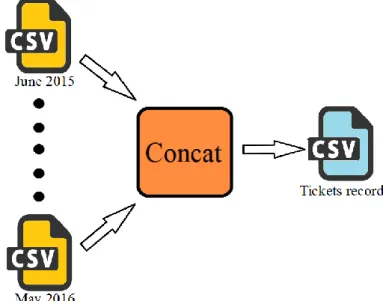
3.3 Data Description ... 48
3.3.1 Tickets dataset ... 49
3.3.2 Items dataset... 50
3.3.3 Stores dataset ... 51
3.4 Application of the Methodology ... 51
3.4.1 Data Pre-processing ... 51 3.4.2 Feature engineering ... 52 3.4.2.1 Features version 1 ... 53 3.4.2.2 Features version 2 ... 54 3.4.2.3 Features version 3 ... 54 3.4.2.4 Features version 4 ... 55 3.4.2.5 Features version 5 ... 55
3.4.3 Clustering Techniques ... 56
3.4.3.1 Selection of the Clustering Technique ... 56
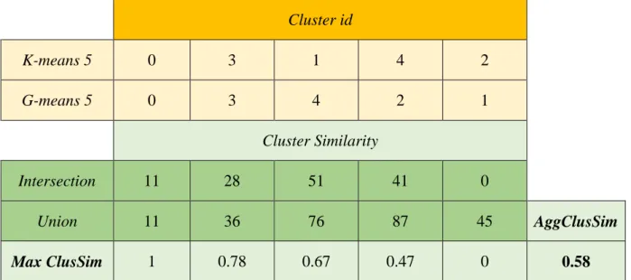
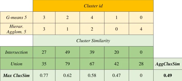
3.4.3.1.1 Clustering composition comparison ... 56
3.4.3.1.2 Structural Validation through Cluster Validation Indexes... 60
3.4.3.2 User Validation through the Interpretation of the Clusters ... 63
3.4.3.2.1 Computing the Relevance of the Variables ... 64
3.4.3.2.2 Generalization of the Variables Using Temporal Relations ... 65
3.4.4 Association discovery ... 68
3.4.5 Results Delivery ... 71
4 Conclusions ... 77
4.1 Difficulties between the scientific world and the company goals ... 78
4.2 Future Work ... 78
References ... 81
Annexes... 87
Annex A: Description of the variables in the three databases ... 87
Chapter 1
Introduction
1.1 Introduction & Motivation
Retail has evolved through its life. Since the common corner store from the 1900s, until the new e-commerce that has shaken the retail world to its core. This changing process has led to a new era of possibilities for the commerce and the consumer.
Consumers nowadays have a wide range of options. In the past, when the consumer had to buy something, he/she only could choose a product from the catalogue of the store. However, with the new era of information and globalization, the list of options has increased exponentially. Products that some years ago were considered as luxury goods nowadays are considered common, and limitations as geography, season or culture are not more an issue. All of this, lead consumers to have a huge variety of possibilities like new products and new companies. This limitless of possibilities to customers is the one that lead companies start to think new strategies to attract new customers or keep its current customers.
This concept is the one that caused this project. The client is a supermarket chain with a wide list of daily consumers. To increase the experience of the customer and increase its incomes as well, the client decided to invest analysing customer's behaviour purchases using knowledge discovery and data mining process [Novak, 2016], and specifically, was interested in finding item’s associations rules within its stores [Association rule, 2017]. This field in retail domain is known as market basket analysis.
Market basket analysis [Kamakura, 2012] encompasses a broad set of analytics techniques aimed at uncovering the associations and connections between specific objects, discovering customer’s behaviours and relations between items. In retail, it is used based on the following idea: if a customer buys a certain group of items, is more (or less) likely to buy another group of items. For example, it is known that when a customer buys beer, in most of the cases, buys chips as well. These behaviours produced in the purchases is what the client was interested in. The client was interested in analysing which items are purchased together in order to create new strategies that improved the benefits of the company and customers experience. There are three main issues where market basket analysis is used.
The first one is the creation of personalized recommendations [Portugal et al., 2015]. This methodology is well known nowadays. During the explosion of the e-commerce,
personalized recommendations has appeared as a part of the marketing process. In a few words, it consists in suggesting items to a customer based on his/her preferences. There are two basic ways to do it. One is suggesting items similar to the ones the customer has purchased in the past (Content-based approach), and the other one is looking for similar customers and recommending items that had purchased the similar customers (Collaborative Filtering approach). Both strategies are often used for companies in order to realize cross-selling and upcross-selling strategies.
The second one is the analysis of spatial distribution in chain stores [R. Kelley & Ming-Long, 2005]. Due the increasing number of products that nowadays exist, physical space in stores has started to be a problem. Increasingly, stores invest money and time trying to find which distribution of items can lead them to obtain more profit. Knowing in advance which items are commonly purchased together, the distribution of the store can be changed to obtain more benefits.
The third one is the creation of discounts and promotions. Based in customer’s behaviour, special sales can be offered. For example, if the client knows which items are often purchased together, he/she can create new offers for his/her customers.
1.2 Definition of the problem and Objectives
The main aim of the project, according to initial thoughts of the client, was the detection and analysis of customers’ purchase behaviour (items purchased together). A basic approach could be the creation of a unique rule list for all the tickets and stores. However, this approach lacked efficiency. For instance, suppose the client wants to create a new offer to a specific store based on the rules discovered. It could happen that the daily clients of the store selected do not have the habit to purchase those items, or those items are not even in the store’s stock. This could be easily solved using another rule from the set of rules. However, this outlined an important concept: stores could have different behaviours, and this fact originated a second aim of the project: the analysis of the possibly different selling behaviour of the stores of the client.
The solution to that problem could be the creation of a store clustering [Pollack, 2016]. Create clusters of stores allow to capture different behaviours. In addition, cluster-local association rules are more realistic and can provide information that is more valuable. The process consisted in create a set of clusters and for each of them, it was selected the store with less distance to the centroid (i.e., the medioid). Then, the association rules of that store were discovered and the results were extrapolated to all the other stores that composed the cluster. With this approach, it was solved the lack of creating a general set of rules for all the stores.
Another issue raised by the client was to define the product level which the association rules should consider. Items belongs to a set of levels. For instance, the item “patatas lays clasicas
170 grs” belongs to family “patatas fritas y fritos”, the section “alimentación seca” and the sector “alimentación y bebidas”. The client uses this taxonomy to classify its items for logistics processes [Logistics, 2017]. However, in this project, the client was not interested in finding rules for items; it was interested in rules based on family level. The client was interested in knowing which product families are purchased together to change its distribution on the stores. In addition, the client was just interested in the items from the sectors: “alimentación y bebidas”, “productos frescos”, “droguería y perfumeria” and “bazar”. Due
that, the entire project was done with the items of these sectors.
1.3 Market Basket Analysis strategy
Once analysed and evaluated the client needs, it was defined the approach of the project. The project was divided in three parts.
The first one was the creation of the store clustering. Using the data provided by the client, a dataset was created, where each instance was a store and the features were structural and behavioural information of that store. With the dataset created, three clustering algorithms were used to obtain the clusters, Hierarchical agglomerative, K-means and G-means. To compare the resulting clusters and analyse the quality of them, two experiments were performed. On the one hand, clusters composition was analysed. To do that, for each pair of algorithms, the stores in its clusters were compared. The aim of this composition similarity comparison was to detect whether different algorithms gave similar results. On the other hand, to evaluate the quality of the structure of the clusters. Four Clusters Validity Indexes (CVIs) were used, Minimum Cluster Separation Index, Maximum Cluster Diameter Index, Dunn Index and Davies-Bouldin Index.
The second one was devoted, once selected the proper algorithm and configuration, to the descriptive analysis of the clusters. Using the cluster to which the store belongs, as a new variable in the dataset, a Random Forest ensemble was applied. Then, the most important attributes were used to perform the descriptive analysis and interpretation of the clusters. A characterisation of each cluster through the most relevant variables, and the centroid computation was done.
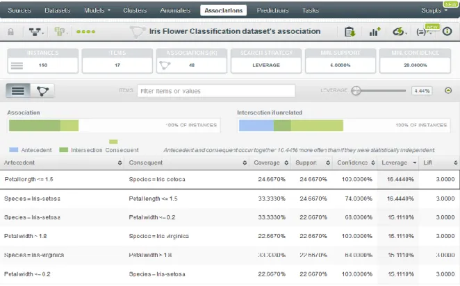
The third one is the analysis of the historic tickets record from one year. For each cluster, the association rules of the stores in it were discovered according to quality measures: Lift and Leverage.
Finally, it was defined that clusters and association rules had to be retrained periodically. Over time, people behaviour change, and new products or new stores can appear. For that reason, data mining models have to be retrained in order to capture new behaviours.
Chapter 2
State of the art
2.1 A Data Science project
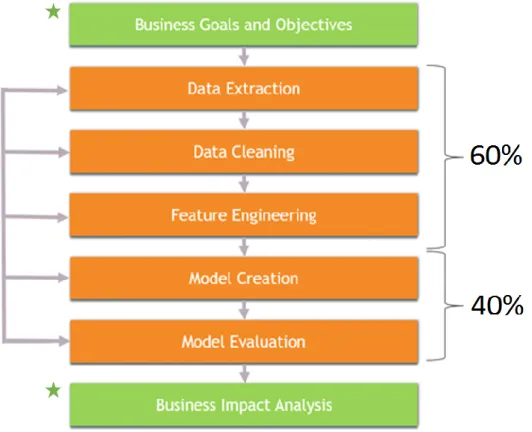
Performing a data science project involves a set of steps to be done. These steps are the skeleton of any data mining/knowledge discovery project. Each one has its own characteristics and objectives, and the sum of all of them, constitute the entire project. The next figure 2.1 is a scheme of the entire process.
Figure 2.1: A data science project skeleton.
Each rectangle represents a step in the project. On the one hand, the steps from Data Extraction until Model Evaluation are related to a common data science project. Those steps could have some come back step among them. On the other hand, the steps Business Goals and Objectives and Business Impact Analysis (star marked) represent the ones where the client has a special impact.
Numbers are time cost approximations of the set of tasks over the total time cost of the project.
Rows are the flux between steps. This is one of the most remarkable characteristics of a data mining project. Flux on traditional projects are sequential, there is just one iteration. However, in this type of problems, the project is developed in several back loops. Therefore, a finished step can be repeated because a new issue or result is obtained.
2.1.1 Business Goals and Objectives
The base of any project is the set of goals and objectives that must be achieved. Decisions and strategies decided in this step, will define the project and the direction where it will be developed.
In this step, the client introduces what he/she expects to achieve using Data Mining techniques. An analysis of the client needs to be performed to understand them, and decide whether they can be achieved using machine learning algorithms or some other technique. If the client needs can be solved using data mining techniques, an approach to the problem is defined and the set of objectives that must be achieved.
2.1.2 Data Extraction
Data extraction is the process of collecting all the available, and presumably interesting, historical data of a company. These data are considered raw because it has not previously received any treatment.
Data extraction is the first step that can be considered part of the data transformation process. Usually this process is a tedious task because companies have data distributed in different sources or databases. In some cases, data is poorly structured or even unstructured. All these aspects convert data extraction process in a hard task.
Nowadays, exist tools prepared to work with this type of problems. Each of them has its own characteristics and methodologies. However, even with this help, the process of collecting data can imply a huge work.
2.1.3 Data Cleaning
Data cleaning is the process of detecting missing values or analysing possible outlier values in the records, and of removing corrupt or inaccurate records from data [Data cleaning, 2017]. Usually, data have errors. These errors can occur being originated from different causes, and the detection of them is vital for the project. Invalid records will imply deterioration of the future model adding noise or false information.
Dara cleaning encompasses the process of removing data which is not relevant or needed as well. Part of the work, is to know which information is relevant or can add value to the algorithms or models used, and treat it for each specific case. Another common situation is that data could be duplicated. Because data emanate from different sources, sometimes the information could be repeated. This provokes an overlap of useless information.
2.1.4 Feature Engineering
Feature engineering is the process of using domain knowledge about the data to create the appropriate features that make machine learning algorithms learn useful patterns from data [Feature engineering, 2017]. This process is fundamental in data mining projects, but it is difficult and expensive. Due this high cost, most of the time of the project is spent in this task. The task consists of finding which features are actually important or needed to add value to the model. This process encompassed the creation and the transformation of features that capture the behaviour and tendencies hidden in the data.
Features used to train a machine learning model affect its performance. As better are the features, better will be the performance. The quality and quantity of features have a huge impact in the model. More than the hyper-parameter configuration of the algorithm, features are the ones that add value to the model. It is worth investing time creating new features, analysing them and transforming data before trying different algorithms.
A complete process of generating an inductive model could be the same as the one used in a cooking recipe. Ingredients would be the dat,a and the algorithm the recipe. If the ingredients are in poor state does not matter that the recipe is the best one of the world, the resulting food will be bad. In the same way, if data has no quality, even with the best algorithm, the results will be bad.
2.1.5 Model Creation
Once obtained the set of features that will be used, the machine learning model is induced /trained from data. Models are feed using the data provided. The dataset, and hence, the learning process can be supervised or unsupervised, and depending on the objective of the problem and the data, supervised or unsupervised machine learning methods are used. A supervised machine learning model uses a supervised dataset, i.e., a dataset which has a special attribute or variable, usually named as the class attribute/variable, which has a label for each observation or instance of the dataset. These labels must be provided by a human expert (here comes the supervised adjective) or obtained by another way. On the contrary, an unsupervised machine learning model uses an unsupervised dataset, i.e., a dataset which has no class attribute/variable at all, and all the observations are unlabelled.
To capture the changing behaviour of the data, machine learning models must be retrained periodically. This period is defined according to the needs of the problem. Alternatively, the machine learning models could be incremental.
2.1.6 Model Evaluation
Model evaluation is the process where the model induced/trained is evaluated using new data. The quality and performance of the model is the result of all the work done through the process. Depending on the type of the model and the type of the target variable, some metrics or others are used to evaluate the quality of the model.
There are two types of evaluation: offline and online. The first one, analyse the performance of a model a priori before deploying it in production. The basic way to do it is with an 80/20 split of the dataset (simple validation) or performing a cross-validation (repeated validation using each fold as test set and the remainder ones as training sets). The second one evaluates the model using real data and analyse its performance.
2.1.7 Business Impact Analysis
The last step in a data mining project is the analysis of the impact that actions had in the problem domain. These actions are executed based on the results obtained through the project.
Companies usually tend to perform projects to obtain a monetary benefit. It can be directly or indirectly. On the one hand, an example of a model used to obtain a direct monetary benefit is one used for churn prediction. It gives a direct income to the company due it prevents to lose clients that would churn. On the other hand, an example of a model used to obtain indirect benefits could be one that group customers based on its behaviours for a posteriori marketing strategy. This model does not feedback with a direct income, but the knowledge of the patterns of those customers can lead to future incomes.
2.2 Data Mining Models
In this project, several data mining models and techniques were used for different tasks. First, descriptive/unsupervised models were used to discover possible groups or clusters of observations (profiles) sharing some interesting features and similar behaviour among themselves. These profiles or clusters should be interpreted by the final users and validated using some structural validation techniques. This structural validation is commonly done in the literature using Cluster Validation Indexes (CVIs).
For the interpretation task of the clusters, some supervised discriminant methods were used to compute the degree of relevance of all the variables. For each cluster, a Random Forest
model, which uses an ensemble of decision trees to make the discrimination process, was used to detect the relevant variables given a concrete cluster.
Finally, once the clusters were interpreted and validated, associative models, and concretely association rules, were used to induce associations among the different variables to get co-occurrence patterns in the data.
Therefore, in the rest of this section, the models and techniques used are described and explained to put them in the adequate context.
2.2.1 Unsupervised/Descriptive Models
There are problems that require discovering the underlying hidden concepts in a dataset or describing the observations/instances by means of obtaining groups or clusters of instances sharing some similarities. Cluster analysis is a Machine Learning task that partitions a dataset and groups together the most similar instances. It separates a set of instances into a number of groups so that instances in the same group, called cluster, are more similar to each other than to those in other groups. Cluster analysis is an unsupervised learning technique. Once the clusters are properly interpreted and validated, it is common to assign a different label to each cluster, creating this way a new qualitative variable in the dataset. Therefore, from then on, the dataset becomes a supervised dataset.
According to the literature [Jain & Dubes, 1988], clustering techniques can be subdivided into partitional clustering techniques and hierarchical clustering techniques by the type of structure imposed on the data. Next, these techniques are described.
2.2.1.1 Partitional Clustering Techniques
A partitional clustering technique generates a single partition of the data in an attempt to recover natural groups present in the data. It tries to obtain a good partition of the observations. The partition is composed by a set of groups or clusters. Thus, this kind of techniques assign each observation to the “best” cluster. This “best” cluster is the one optimizing certain criterion (minimisation of the square sum of distances of the observations to the centroids of the clusters, etc.). Either these algorithms require the number of clusters to be obtained, namely k, or some threshold value (classification distance) used to decide whether an observation belongs to a forming cluster or not.
Partitional clustering methods are especially appropriate for the efficient representation and compression of large databases, and when just one partition is needed.
Most popular techniques are the K-means clustering algorithm and the Nearest-Neighbour clustering technique. Next, these algorithms and a variation of K-means algorithm will be described.
2.2.1.1.1 K-means Clustering
One of the most popular partitional clustering algorithms is the K-means clustering algorithm [MacQueen, 1967]. Starting with a randomly initial partition, it explodes the idea of changing the current partition to another one decreasing the sum of squares of distances of the observations to the centroids of the clusters. It converges, possibly to a local minimum, but in general can converge fast in a few iterations. It has a main parameter k, which is the number of desired clusters.
The general scheme of the algorithm is as follows:
Algorithm k-means (k)
Assign randomly k observations as the centres of the k clusters
while any observation changes its cluster membership do
Assigning each observation to its closest cluster centre Compute new cluster centres as the centroids of the clusters
endwhile
2.2.1.1.2 G-means Clustering
Sometimes is hard to know in advance how many clusters can be identified in a dataset or simply it is not desired to force the algorithm to output a specific number of clusters. Gaussian-means (means) [Hamerly & Elkan, 2003] was designed to solve this issue. G-means use a special technique for running K-G-means multiple times while adding centroids in a hierarchical way. G-means has the advantage of being relatively resilient to covariance in clusters and has no need to compute a global covariance. The G-means algorithm starts with a small number of k-means centres, and grows the number of centres. Each iteration of the algorithm splits into two those centres whose data appear not to come from a Gaussian distribution. Between each round of splitting, k-means is run on the entire dataset and all the centres to refine the current solution.
The test used is based on the Anderson-Darling statistic [Anderson & Darling, 1954]. This one-dimensional test has been shown empirically to be the most powerful normality test that is based on the empirical cumulative distribution function (ECDF).
The general scheme of the algorithm is as follows:
Algorithm G-means (X, α)
Let C be the initial set of centers (usually C ← {x¯}, i.e., k=1)
repeat
C ← kmeans(C, X)
Let {xi|class(xi) = j} be the set of datapoints assigned to center cj
for eachcj C do
Use a statistical test to detect if {xi|class(xi) = j} follow a Gaussian distribution
(at conf. level α)
if the data look Gaussian then keep cj
else replace cj with two centers
endif endfor
until no more centers are added
2.2.1.1.3 Nearest-Neighbour Clustering
A natural way to define clusters is by utilizing the property of nearest neighbours; an observation should usually be put in the same cluster as its nearest neighbour. Two observations should be considered similar if they share neighbours.
One of the most used clustering algorithm which is based on the nearest neighbour idea is due to [Lu & Fu, 1978], where the user specifies a threshold, t, on the nearest-neighbour distance. If new observations are at a less distance from its nearest neighbour than t, then they are assigned to the same cluster than its nearest neighbour.
The general scheme of the algorithm is as follows:
Algorithm Nearest-Neighbour (t)
Let number of clusters (k), k = 1 Assign observation x1 to cluster C1
while not all observations are processed do
Find the NN of observation Xi among the observations already assigned to clusters
Let di,NNm denote the distance from Xi to its nearest neighbour (NNm) in cluster m if di,NNmtthen assign Xi to Cm.
else set k = k + 1;
assign X¡ to a new cluster Ck endif
2.2.1.2 Hierarchical Clustering Techniques
A hierarchical clustering process is a nested sequence of partitions. Hierarchical clustering is a general family of clustering algorithms that build nested clusters by merging or splitting them successively. This hierarchy of clusters is represented as a tree, (named as dendrogram). A dendrogram is a special type of tree structure that provides a convenient picture of a hierarchical clustering. A dendrogram consists of a rooted binary tree, where the nodes represent clusters. Lines connecting nodes represent clusters which are nested into one another. Cutting horizontally a dendrogram creates a clustering. Figure 2.2 provides a simple example of a dendrogram.
The root of the tree is the unique cluster (conjoint cluster) that gathers all the samples; the leaves being the clusters with only one sample (disjoint clusters). Hierarchical clustering techniques are useful when more than one partition is needed and/or when taxonomies are required like in Medical, Biological or Social Sciences. Anyway, Dendrograms are impractical with more than a few hundred observations.
Figure 2.2. A simple example of a dendrogram from a hierarchical clustering process Techniques for hierarchical clustering can be divided into two basic paradigms: agglomerative (bottom-up) and divisive (top-down) approaches. All the agglomerative and some divisive methods (viewed in a bottom-up direction) possess a monotonicity property: the dissimilarity between merged clusters is an increasing monotonic function regarding the level of the merger. Therefore, the dendrogram can be plotted so that the height of each node is proportional to the value of the intergroup dissimilarity between its two children.
2.2.1.2.1 Agglomerative/Ascendant Techniques
An agglomerative or ascendant hierarchical clustering place each object in its own cluster, and gradually merges these atomic clusters into larger and larger clusters until all objects are in a single cluster. The pair chosen at each step for merging consist of the two clusters with the smallest intergroup dissimilarity (distance). There are several methods implementing this principle. Their difference relies in how they compute the distances (similarities) between the clusters and/or the observations
The general algorithmic scheme for hierarchical agglomerative/ascendant clustering technique [Johnson, 1967] is as follows:
Algorithm Hierarchical agglomerative clustering
Let N be the number of observations to be clustered
Start by assigning each observation to a cluster (N clusters)
Let the distances between the clusters be the distances between the observations they contain
whilenot all observations are clustered into a single cluster of size N do
Find the closest pair of clusters // differential step of algorithms Merge them into a single cluster
Compute distances between the new cluster and each of the old clusters
endwhile
The different variations of the hierarchical ascendant clustering techniques rely on the step of finding the closest (more similar) pair of clusters. Main used algorithms are known as single-linkage clustering, complete-linkage clustering, average-linkage clustering, centroid-linkage clustering and Ward’s method:
● Single-linkage clustering (also called the connectedness or minimum method) considers the distance between one cluster and another cluster to be equal to the
shortest distance from any member of one cluster to any member of the other cluster. ● Complete-linkage clustering (also called the diameter or maximum method), considers the distance between one cluster and another cluster to be equal to the greatest distance from any member of one cluster to any member of the other cluster.
● Average-linkage clustering, considers the distance between one cluster and another cluster to be equal to the average distance from any member of one cluster to any member of the other cluster.
● Centroid-linkage clustering, considers the distance between one cluster and another cluster to be equal to the distance between the centroids of each cluster.
● Ward’s method (also called the minimum variance method) [Ward, 1963], which merges in a new cluster (t), the pair of clusters (p, q) minimizing the change in the square-error of the entire clustering ∇𝐸𝑝𝑞2 = 𝑒
𝑡2− 𝑒𝑝2− 𝑒𝑞2. The square-error of the
entire clustering is the sum of the square-errors for the individual clusters (i.e., sum of squared distances to the centroid for all the observations in a cluster).
The general complexity for agglomerative clustering is O(n2 log(n)) [Rokach & Maimon,
2005], but for some special cases, optimal efficient agglomerative methods of complexity
O(n2) are known: SLINK [Sibson, 1973] for single-linkage clustering and CLINK [Defays, 1977] for complete-linkage clustering.
2.2.1.2.2 Divisive/Descendent Techniques
Divisive or descendent hierarchical clustering reverses the process by starting with all objects in one cluster and recursively divide one of the existing clusters into two daughter clusters at each iteration in a top-down procedure. The split is chosen to produce two new clusters with the largest intergroup dissimilarity (distance).
In the general case, divisive clustering techniques have a complexity of O(2n−1) [Everitt, 2011]. For that reason, divisive methods are not very popular, and this approach has not been studied as extensively as agglomerative methods in the clustering literature. The existent algorithms propose some heuristic in order not to generate all possible splitting combinations. One of the first divisive algorithm in the literature was proposed in [Macnaughton-Smith et al., 1965]. It begins by placing all observations in a single cluster G. It then chooses that observation whose average dissimilarity from all the other observations is largest. This observation forms the first member of a second cluster H. Then, it moves to the new cluster H the observations in G whose average distance from those in G is greater than the average distance to the ones in the new cluster H. The result is a split of the original cluster into two children clusters, the observations transferred to H, and those remaining in G. These two clusters represent the second level of the hierarchy. Each successive level is produced by applying this splitting procedure to one of the clusters at the previous level.
Other divisive clustering algorithm was published as the DIANA (DIvisive ANAlysis Clustering) algorithm [Kaufman & Roussew, 1990]. DIANA follows the same strategy proposed by Macnaughton-Smith, but chooses the cluster with the largest diameter (i.e., the one maximizing the distance among its member observations). A possible alternative could be to choose the one with the largest average dissimilarity among its member observations. An obvious alternate choice is k-means clustering with k = 2, [Steinbach et al., 2000] but any other clustering algorithm producing at least two clusters can be used, provided that the splitting sequence possesses the monotonicity property required for a dendrogram
representation.
2.2.1.3 Clustering Validation Techniques
Once a clustering technique has been applied, the resulting set of clusters must be validated to ensure that the clusters are structurally well formed, and to get the underlying meaning of the clusters. Usually, the real partition of the data is unknown and, therefore, the results from a clustering process cannot be compared with a reference partition by computing misclassification indexes, as in the case of supervised learning.
2.2.1.3.1 Structural Validation of Clusters
Cluster structural validation in clustering field is an open problem. In the literature, most of used techniques for evaluating the clustering results are based on numerical indexes, which
evaluate the validity of the resulting partition from different points of view, known as Cluster Validity Indexes (CVI). A wide number of CVIs can be found in literature and some surveys comparing several CVIs [Halkidi et al., 2001]. However, there are currently no clear guidelines for deciding which is the most suitable index for a given dataset [Brun et al., 2007]. In fact, there is not an agreement among those indexes, but it seems clear that each one can give some information about a different property of the partition like homogeneity, compactness of classes, variability, etc. All these CVIs refer to structural properties of the partition, which are context-independent, and the evaluation based on them is mainly made in terms of the cluster' topology.
Most common CVIs in the literature are: ● Entropy index
● Maximum Cluster Diameter index (∆) ● Widest Gap index (wg )
● Average Within-Cluster Distance index (W) ● Within Cluster Sum of squares index (WSS) ● Average Between-Cluster Distance index (B) ● Minimum Cluster Separation index(δ)
● Separation index (Sindex) ● Dunn index (D)
● Dunn-like index
● Calinksi-Harabasz index (CH)
● Normalized Hubert Gamma Coefficient (Γˆ) ● Silhouettes index
● Baker and Hubert index (BH) ● Within Between Ratio index (WBR) ● C-index
● Davies-Bouldin index (DB)
In a recent work [Sevilla-Villanueva et al., 2016], it was outlined that indexes evaluate a reduced set of characteristics of a partition. Thus, all indexes can be grouped around 4 basic concepts:
● Indexes measuring compactness of clusters: Diameter (∆), wg, W, WSS.
● Indexes measuring separation between clusters: B, Separation (δ), Sindex.
● Indexes measuring relationships between compactness and separation: CH,
Silhouettes, Γˆ, BH, WBR, C-Index, DB, and also D, Dunn-like.
● Indexes measuring chaos in the clusters: Entropy.
Therefore, it would be a good strategy to select one index from a different family to evaluate different properties of the clustering result. In the project, the following four indexes were selected to be used:
Maximum Cluster Diameter (∆) [Hennig and Liao, 2010] is the maximum distance between any two points that belongs to the same cluster.
∆ = max 𝐶𝑖∈𝑃 ∆𝐶𝑖 ∆𝐶𝑖= max𝑜 1,𝑜2∈𝐶𝑖 𝑑(𝑜1, 𝑜2)
Minimum Cluster Separation (δ) is the minimum distance between any two objects that do not belong to the same cluster. In other words, it is defined by the lower separation among all the clusters. 𝜕 = min 𝐶1,𝐶2∈𝑃 𝜕𝐶1,𝐶2 𝜕𝐶1,𝐶2=𝑜 min 1∈𝐶1,𝑜2∈𝐶2 𝑑(𝑜1, 𝑜2)
Dunn Index (D) is a cluster validity index for crisp clustering proposed in [Dunn, 1974]. It attempts to identify ”compact and well separated clusters”
𝐷 =𝜕 ∆= min 𝐶1,𝐶2∈𝑃𝜕𝐶1,𝐶2 max 𝐶𝑖∈𝑃∆𝐶𝑖
Davies-Bouldin Index (DB) [Davies & Bouldin, 1979] is a cluster relation of compactness and separation measure. The overall index is defined as the average of indexes computed from each individual cluster. An individual cluster index is taken as the maximum pairwise comparison involving the cluster and the other clusters in the solution.
𝐷𝐵 = 1 𝑚∑𝐶′∈𝑃,𝐶′≠𝐶max ( 𝑠𝑝𝐶+ 𝑠𝑝𝐶′ 𝑑𝑝(𝐶, 𝐶′) ) 𝐶∈𝑃 Where 𝑑𝑝(𝐶, 𝐶′) = √∑𝐾𝑘=1|𝑋̅̅̅̅̅ − 𝑋𝐶𝑘 ̅̅̅̅̅|𝐶′𝑘 𝑝 𝑝 and 𝑠𝑝𝐶 = √ ∑𝑜𝑖∈𝐶𝑑𝑝(𝑜𝑖,𝑜𝑖𝑐)𝑝 𝑛𝐶 𝑝
Where, 𝑜𝑖𝑐is the barycenter of the cluster C defined as 𝑜𝑖𝑐 = (𝑥̅̅̅̅, … , 𝑥𝐶1 ̅̅̅̅) 𝐶𝑘
2.2.1.3.2 Expert Validation of Clusters
In addition to the structural validation of the clusters, it is very important to make a qualitative validation of the clusters. Usually, the experts make this kind of validation. This validation process consists to carefully look at the composition of the obtained clusters, analyse them, and try to get an interpretation of each one of the clusters.
This interpretation process can be done through some data summarisation techniques, like the computation of the cluster centroids. A cluster centroid is a prototype showing the most frequent characteristics of the observations belonging to that cluster. This information is very important to illustrate how is the general profile of the observations belonging to a cluster. A centroid is a virtual observation, which is the geometrical centre of the set of observations. It has the same number and type of components than the observations, and usually has the average value of the numerical variables, the mode of qualitative variables, etc. IT provides a very useful information of the prototypical kind of observations of a cluster (low values of variable X1, high values of variable X2, etc.)
In addition, several graphical visualizations of data can help to the interpretation of the clusters (histograms, tables, bivariate plots, letter plots, etc.). All these graphics can help to identify the characteristics of each one of the clusters.
2.2.2 Supervised Discriminant Models
Another common problem in Machine Learning is to obtain a discriminant model from a supervised dataset. Discriminant models are able to discriminate or predict the class label of a new unlabelled instance. Discriminant models are also called classifier models or systems in the literature.
There are several kinds of discriminant methods like Support Vector Machines, Decision Trees, Classification Rules, Bayesian discriminant methods, Case-Based Classifiers, etc. In addition, in the literature there is the approach of working with an ensemble of discriminant methods. As in this project work, Decision Trees, and some ensemble of classifiers approach, concretely Random Forests were used. All these techniques are detailed a bit in the next subsections.
2.2.2.1 Decision Trees
A decision tree is a hierarchical structure (a tree), which can model the decision process of deciding to which class belongs a new example of a concrete domain. In a decision tree, the internal nodes represent qualitative attributes, or discretized numerical ones in some approaches. For each possible value of the qualitative attribute, there is a branch. The leaves of the tree have the qualitative prediction of the attribute that acts as a class label.
Decision Trees has some advantages over other discriminant models. The final model, the tree, is easily interpretable by an expert or end user to understand the decision process, which ends assigning a label to a new unlabelled instance. Another interesting point is that at the same time that the decision tree is constructed, the attributes that have not been used in the building of the tree, are not necessary for a discrimination process. This fact probably means that those unused attributes are not very important. This way, using a decision tree has the
benefit of performing an internal feature selection process as an integral part of the procedure. They can manage the presence of irrelevant predictor attributes.
There are different techniques to induce a decision tree from a supervised training dataset. All methods use a top-down recursive procedure with a greedy strategy to select the adequate attribute at each node. The strategy tries to select the most discriminant attribute at each step. The discrimination among the different classes is maximized, when the level of separation or skew among the different classes in a given node is maximized.
The difference among the methods relies on how to estimate which is the most discriminant one. Most common methods in the literature are:
● ID3 method [Quinlan, 1983; Quinlan, 1986] ● CART method [Breiman et al., 1984] ● C4.5 method [Quinlan, 1993]
The measures used to compare different decision trees are: the compactness of the tree, the predictive accuracy of the tree, the generalization ability of the tree (scalability). In addition, some approaches propose pruning techniques to reduce the size of the tree and try avoiding overfitting problems.
2.2.2.1.1 Information Gain Methods
One of the most well-known method for inducing a decision tree is the ID3 [Quinlan, 1983; Quinlan 1986] method. On each iteration of the algorithm, it selects the best attribute according to the Information Gain criteria.
The Information Gain criteria is based on the concept of Entropy from information theory. The criteria selects the attribute, which maximizes the information gain. Thus, the ID3 algorithm needs to assess the information gain provided by the use of each one of the considered attributes. The Entropy function measures the ability of each attribute to split the instances in the possible values of the attribute in the best pure (discriminant) form. Purity means that if all instances having the same value for the attribute belongs to the same label is a better attribute than others that are mixing several instances belonging to different labels.
𝐺𝑎𝑖𝑛(𝑋, 𝐴) = 𝐼𝑛𝑓𝑜(𝑋) − 𝐼𝑛𝑓𝑜(𝑋, 𝐴)
Where X is the set of all instances to be discriminated at each node, and k is the number of different labels of the class attribute.
𝐼𝑛𝑓𝑜(𝑋) = 𝐻(𝑋) = − ∑ 𝑝𝑥∈𝐶𝑖∗ log2𝑝𝑥∈𝐶𝑖
𝑘 𝑖=1
𝐼𝑛𝑓𝑜(𝑋, 𝐴) = ∑ 𝑝𝑥∈𝑉𝑎𝑙𝑢𝑒𝑗(𝐴)∗ 𝐼𝑛𝑓𝑜({𝑥|𝑥 ∈ 𝑉𝑎𝑙𝑢𝑒𝑗(𝐴)})
𝑣 𝑗=1
is the amount of information needed to arrive to a perfect classification using the corresponding attribute A.
The value of the entropy lies between 0 and log(k). The value is log(k), when the instances are perfectly balanced among the different classes. This corresponds to the scenario with maximum entropy. The smaller the entropy, the greater the separation in the data.
It selects the attribute which has the smallest entropy (or largest information gain) value. The set X is then split by the selected attribute to produce subsets of the data. The algorithm recursively continues on each subset, considering only attributes never selected before.
This Information Gain measure is biased to select attributes with large number of possible values. In order to overcome this bias, Quinlan [Quinlan, 1993] proposed the C4.5 method which uses an extension to information gain known as gain ratio. It applies a kind of normalization to information gain using a split information value. The split information value
represents the potential information generated by splitting the training data set X into v
partitions, corresponding to the v possible values of the attribute A.
𝑆𝑝𝑙𝑖𝑡𝐼𝑛𝑓𝑜𝐴(𝑋) = − ∑ 𝑝𝑥∈𝑉𝑎𝑙𝑢𝑒𝑗(𝐴)∗ log2(𝑝𝑥∈𝑉𝑎𝑙𝑢𝑒𝑗(𝐴))
𝑣 𝑗=1
The GainRatio is defined as follows:
𝐺𝑎𝑖𝑛𝑅𝑎𝑡𝑖𝑜(𝑋, 𝐴) = 𝐺𝑎𝑖𝑛(𝑋, 𝐴) 𝑆𝑝𝑙𝑖𝑡𝐼𝑛𝑓𝑜𝐴(𝑋)
At each node of the tree, C4.5 chooses the attribute of the data that most effectively splits its set of samples into subsets according to the Normalized Information Gain or Gain Ratio. The attribute with the highest Gain Ratio is chosen.
The C4.5 method has been implemented in the J4.8 method in the software WEKA. In next evolutions of the method, Quinlan proposed the C5.0 method, where the most significant feature unique to C5.0 is a scheme for deriving rule sets.
2.2.2.1.2 Impurity Measure Method
Another well-known method is the CART method (Classification And Regression Trees) [Breiman et al., 1984], which base Impurity measure. For example, if p1 ... pk is the fraction
of the instances belonging to the k different classes in a node N, then the Gini-index of impurity Gini(X) of the current node is defined as follows:
𝐺𝑖𝑛𝑖(𝑋) = 1 − ∑ 𝑝𝑥∈𝐶𝑖
𝑘 𝑖=1
Where X is the set of all instances to be discriminated at each node, and k is the number of different labels of the class attribute.
The value of Gini(X) lies between 0 and 1 − 1/k. The smaller the value of Gini(X), the greater the separation. In the cases where the classes are evenly balanced, the value is 1 − 1/k.
The Gini Index considers only a binary split for each attribute A, say X1 and X2. The Gini
index of X given that partitioning is a weighted sum of the impurity of each partition:
𝐺𝑖𝑛𝑖(𝑋, 𝐴) = |𝑋1|
|𝑋| ∗ 𝐺𝑖𝑛𝑖(𝑋1) + |𝑋2|
|𝑋| ∗ 𝐺𝑖𝑛𝑖(𝑋2)
Finally, the attribute that maximizes the reduction in impurity is chosen as the splitting attribute.
∆𝐺𝑖𝑛𝑖(𝐴) = 𝐺𝑖𝑛𝑖(𝑋) − 𝐺𝑖𝑛𝑖(𝑋, 𝐴)
2.2.2.2 Ensemble Methods
In the literature, there are several works proposing the use of a set of discriminant/classifier models. The aim is to build a discriminant/classifier model by combining the strengths of a collection of simpler base models. There are several ways of implementing this idea. Some approaches are based on resampling the training set, others on using different discriminant/classifier methods, others on varying some parameters of the classifier methods, etc. Finally, the ensemble of methods is used to combine the output of each classifier, i.e., the predicted label, by means of a (weighted) majority voting.
In next subsections, the most common approaches are detailed: bagging, boosting and random forests.
2.2.2.2.1 Bagging
The Bagging (Bootstrap Aggregating) strategy [Breiman, 1996] propose to create ensembles by repeatedly and randomly resampling the training data. Given a training set of size n, create
m samples of size n by drawing n examples from the original data, with replacement. These are referred to as bootstrap samples. Each bootstrap sample will contain different training examples, and the rest are replicates. For each sample, the classifier method is used to induce one model. At the testing step, all models are used, and their output labels are combined in a majority vote scheme.
This approach has often been shown to provide better results than single models in certain scenarios. This approach can reduce the variance of classifiers improving the accuracy, because of the specific random aspects of the training data. Decreases error by decreasing the variance in the results due to unstable learners (like decision trees) whose output can change dramatically when the training data is slightly changed.
2.2.2.2.2 Boosting
Boosting [Freund, 1995] is a common technique used in classification. The idea is to focus on successively difficult instances of the data set, to create models that can classify these instances more accurately, and then use the ensemble scores over all the components. A holdout approach is used to determine the incorrectly classified instances of the data set. Thus, the idea is to sequentially determine better classifiers for more difficult instances, and then combine the results to obtain a meta-classifier, which works well on all the dataset. To focus on difficult instances, they are given weights. At each iteration, a new hypothesis is learned and the examples are reweighted to focus the system on examples that the most recently learned classifier got wrong.
General boosting algorithm can be expressed as follows:
Algorithm Boosting
Set all examples to have equal uniform weights
fort from 1 to T do
Learn a hypothesis, ht from the weighted examples
Decrease the weights of examples ht classifies correctly
endfor
Base (weak) learner must focus on correctly classifying the most highly weighted examples while strongly avoiding over-fitting. During testing, each of the T hypotheses get a weighted vote proportional to their accuracy on the training data.
One of the most used boosting approach is the AdaBoost (Adaptive Boosting) algorithm [Freund & Shapire, 1997], for building ensembles, that empirically improves generalization performance.
2.2.2.2.1 Random Forests
Random forests [Breiman, 2001] is a method that proposes to use sets of unpruned decision trees aiming to reduce the error of the single classifiers. Each decision tree is built splitting at each node using a random selection of features and the training data for each tree is a bootstrap sample of the training data.
A number m is specified much smaller than the total number of attributes M (e.g., m = sqrt
(M) or m = int (log2 M +1)). At each node, m attributes are selected at random out of the M. The split used is the best split, according to the criteria used (information gain, gain ratio, Gini index of impurity, etc.), on these m attributes.
At the testing step of unclassified instances, final classification is done by majority vote across the trees. Usually, error rates compare favourably to AdaBoost. It is more robust with respect to noise, and efficient on large data.
Random forests are closely related to bagging, and in fact bagging with decision trees can be considered a special case of random forests, in terms of how the sample is selected (bootstrapping). In addition, they provide an estimation of the importance of features in determining classification.
2.2.3 Associative Models
In the same way that descriptive models try to find relationships among the instances of a database, there are associative models, which aim to find some relationship among the variables in a dataset. There are problems that require finding meaningful relationships among variables in large datasets across thousands of values, e.g., discovering which products are buy together by customers (i.e., market basket analysis), finding interesting web usage patterns, or detecting software intrusion. These problems can be solved using Associative models. Among the associative models, most commonly used methods are Association Rules techniques, Qualitative Reasoning models, and other statistical methods like Principal Component Analysis (PCA), etc. Association Rule techniques have been used in this work for its easiness of interpretation by the experts. For that reason, they are described in the next subsection.
2.2.3.1 Association Rules
The main goal of the Association Rules technique is to obtain a set of association rules which express the correlation among attributes, from a database of item transactions. These techniques were originated in the field of Knowledge Discovery in large databases. Thus, accordingly, the common terminology talks about transactions, databases, and items in the transactions, because these techniques were first applied to the market basket analysis domain, and the transactions were composed of the different items bought by a customer. Given a database consisting of a set of transactions D = {t1, t2, … , tn}, and given I={i1, ...,
in} be a set of n attributes called items.
Each transaction in D has a unique transaction ID and contains a subset of the items in I: t1: i2, i3, i4, i6, i9
t3: i2, i4, i5, i6
t4: i1, i3, i4, i8, i9, i10
. . .
tn: i3, i4, i6, i9
The issue is to obtain common patterns of co-occurrence of the same items along the database. Of course, in order that the co-occurrences found in the database have some interest, the database should have enough number of transactions in order that the co-occurrence appear a sufficient number of times. This minimum number of times required for a co-occurrence is named as the minimum support (minsup) of the rule expressing the co-occurrence.
For instance, the following common patterns can be obtained from the previous database: i2, i4 i4, i9 i2, i4, i9 i3, i4, i9 i3, i4, i6, i9 ...
From a common pattern, several association rules can be generated. An association rule is defined as an implication of the form:
X ⇒ Y
where X, Y I and X Y =
Every rule is composed by two different sets of items, also known as itemsets, X and Y. X is called the antecedent or left-hand-side (LHS) of the rule and Y is called the consequent or right-hand-side (RHS) of the rule.
For instance: i2⇒ i4 i4⇒ i2 i4⇒ i9 i9⇒ i4 i2⇒ i4 ∧ i9 i4⇒ i2 ∧ i9 i9⇒ i2 ∧ i4 i2∧ i4 ⇒ i9 i2∧ i9 ⇒ i4 i4∧ i9 ⇒ i2 i3∧ i4 ⇒ i9 i3∧ i9 ⇒ i4 i4∧ i9 ⇒ i3 i3∧ i4 ∧ i6 ⇒i9 i3∧ i4 ∧ i9 ⇒i6 i3∧ i6 ∧ i9 ⇒i4 i3∧ i4 ∧ i6 ⇒i9 i3∧ i4 ⇒i6 ∧ i9 i3∧ i6 ⇒i4 ∧ i9 . . . . . .
In the general case of application of association rules, an item is an attribute-value pair, and the term itemset is the combination of items that have a minimum specified support (minsup). Next, the main concepts related to association rules are defined:
● Support of an itemset [Agrawal et al., 1993]
(instances) in the database, which contains the itemset X.
𝑠𝑢𝑝𝑝(𝑋) = |{𝑡 ∈ 𝑇|𝑋 ⊆ 𝑡}| (absolute definition)
𝑠𝑢𝑝𝑝(𝑋) = |{𝑡∈𝑇|𝑋 ⊆ 𝑡}|
|𝑇| (relative definition)
● Support of a rule [Agrawal et al., 1993]
The support value of a rule, X ⇒ Y, with respect to T is defined as the percentage of all transactions (instances) in the database, which contains the itemset X and the itemset Y.
𝑠𝑢𝑝𝑝(𝑋 ⇒ 𝑌) =𝑠𝑢𝑝𝑝(𝑋 ∪ 𝑌) |𝑇|
● Coverage of a rule
Coverage is sometimes called antecedent support or LHS support. It measures how often a rule, X ⇒Y, is applicable in a database.
𝑐𝑜𝑣𝑒𝑟𝑎𝑔𝑒(𝑋 ⇒ 𝑌) = 𝑠𝑢𝑝𝑝(𝑋)
● Confidence/Strength of a rule [Agrawal et al., 1993]
The confidence value of a rule, X ⇒ Y, with respect to a set of transactions T, is the proportion of the transactions that contains X, which also contains Y.
𝑐𝑜𝑛𝑓(𝑋 ⇒ 𝑌) =𝑠𝑢𝑝𝑝(𝑋 ∪ 𝑌) 𝑠𝑢𝑝𝑝(𝑋)
● Leverage/Piatetsky-Shapiro Measure (PS) of a rule [Piatetsky-Shapiro, 1991]
Leverage value of a rule, X ⇒ Y, measures the difference between the probability of the rule and the expected probability if the items were statistically independent.
𝑙𝑒𝑣𝑒𝑟𝑎𝑔𝑒(𝑋 ⇒ 𝑌) = 𝑠𝑢𝑝𝑝(𝑋 ⇒ 𝑌) − 𝑠𝑢𝑝𝑝(𝑋) ∗ 𝑠𝑢𝑝𝑝(𝑌)
It ranges from [-1, +1] indicating 0 the independence condition.
● Lift/Interest of a rule [Brin et al., 1997]
Lift value of a rule, X ⇒ Y, measures how many times more often X and Y occur together than expected if they were statistically independent.
𝑙𝑖𝑓𝑡(𝑋 ⇒ 𝑌) = 𝑠𝑢𝑝𝑝(𝑋 ∪ 𝑌)
𝑠𝑢𝑝𝑝(𝑋) ∗ 𝑠𝑢𝑝𝑝(𝑌)=
𝑐𝑜𝑛𝑓(𝑋 ⇒ 𝑌) 𝑠𝑢𝑝𝑝(𝑌)
It ranges from [0, +∞] where a lift value of 1 indicates independence between X and Y, and higher values indicates a co-occurrence pattern.
The different methods to induce the association rules are interested in rules with a minimum support (minsup) to outline a repetitive co-occurrence pattern, and with high confidence, meaning that the rules are highly accurate (both antecedent and consequent of the rule are satisfied). Also, high values of lift are desirable to indicate a co-occurrence pattern strength. Most well-known methods in the literature are the following:
● Apriori algorithm [Agrawal & Srikant, 1994] was one of the earliest association rules method. In fact, the Apriori algorithm computes just the large itemsets which their support is higher than the minimum support (minsup) threshold. It uses a breadth-first search strategy to generate the itemsets: starting from large 1-itemsets, it computes afterwards large 2-itemsets, then large 3-itemsets and so on until the maximum number of attributes available. It uses a candidate generation function, which filters impossible large k-itemsets candidates, because they have subsets of large k-1-itemsets, which do not have a minimum support.
After the Aprori algorithm, the candidate rules must be generated trying all the possible combinations of the items in the antecedent or the consequent of the rule. The rules are filtered, and just only the ones with a confidence value higher than the minimum confidence bound are shown.
● Eclat (Equivalence CLAss Transformation) [Zaki, 2000; Zaki et al., 1997] is a depth-first search algorithm using set intersection. It uses a vertical tid-list database format where it associates with each itemset, a list of transactions in which it occurs. All frequent itemsets can be enumerated via simple tid-list intersections. In addition, a lattice-theoretic approach to decompose the original search space (lattice) into smaller pieces (sublattices) which can be processed independently in main-memory is used. Eclat uses a prefix-based equivalence relation for the decomposition of the lattice and a bottom-up strategy for enumerating the frequent itemsets within each sublattice. Eclat requires only a few database scans, minimizing the I/O costs, and it is suitable for both sequential as well as parallel execution with locality-enhancing properties. The association rules are generated after the Eclat method, using the same procedure as Aprori and other methods.
● FP-growth (Frequent Pattern growth) [Han et al., 2004; Han et al., 2000] proposed a novel frequent-pattern tree structure (FP-tree), which is an extended prefix-tree structure for storing compressed, crucial information about frequent patterns, and develop an efficient FP-tree based mining method, FP-growth, for mining the complete set of frequent patterns by pattern fragment growth. Efficiency is achieved with a large database, which is compressed into a condensed, smaller data structure, FP-tree which avoids costly, repeated database scans. The FP-tree-based mining adopts a pattern-fragment growth method to avoid the costly generation of a large number of candidate sets. Moreover, a partitioning-based, divide-and-conquer method is used to decompose the mining task into a set of smaller tasks for mining confined