Market basket analysis in retail

(1)

Market Basket Analysis

in Retail

Gerard Reig Grau

January/February 2017

Advisor: Andrés González, CleverData

Tutor: Miquel Sànchez-Marrè, Dept. of Computer Science (UPC)

MASTER IN ARTIFICIAL INTELLIGENCE

FACULTAT D’INFORMÀTICA DE BARCELONA (FIB)

FACULTAT DE MATEMÀTIQUES (FM)

ESCOLA TÈCNICA SUPERIOR D’ENGINYERIA (ETSE)

UNIVERSITAT POLITÈCNICA DE CATALUNYA (UPC) – BarcelonaTech

UNIVERSITAT DE BARCELONA (UB)

(2)

(3)

Abstract

In this Master Thesis memory will be described a full end-to-end data science project performed in CleverData, a successful start-up specialized in machine learning techniques and analytics tools. Over all its capacities, it offers a huge variety of solutions to nowadays business needs from different domains.

This project was performed for one of its client, an important retail company from Spain. It consist of analysing the market basket of customers. Thus, the main goal is to find which items are purchased together in their stores.

Through the memory, the reader will see how, step by step, the project grows. Since the first step of defining objectives, until the last one of results delivery. Moreover, the reader will see one of the most promising tools used for machine learning as a service nowadays, BigML. At the end of the project, the reader will have a general idea how data science projects are structured, and how machine learning can be used to solve real problems in today’s companies.

(4)

(5)

2.2 BigML . . . 14 2.2.1 Supervised Learning . . . 15 2.2.1.1 Sources . . . 16 2.2.1.2 Datasets . . . 17 2.2.1.3 Models . . . .17 2.2.1.4 Ensembles . . . 19 2.2.1.5 Logistic Regressions . . . 21 2.2.1.6 Predictions . . . .21 2.2.1.7 Evaluations . . . 22 2.2.2 Unsupervised Learning . . . 22 2.2.2.1 Clusters . . . 22 2.2.2.2 Anomalies . . . 23 2.2.2.3 Associations . . . 24 2.3 Models Learning . . . 25 2.3.1 Clustering Models . . . 25 2.3.1.1 K-means . . . 26 2.3.1.2 G-means . . . 26 2.3.2 Association Discovery . . . .27 2.3.2.1 Association Measures . . . 29

(6)

3.3 Data . . . 33 3.3.1 Tickets dataset . . . 34 3.3.2 Articulos dataset . . . 36 3.3.3 Puntos Venta dataset . . . .38

3.4 Application of the Methodology . . . 40

3.4.1 Clustering . . . 40 3.4.1.1 Version 1 . . . .41 3.4.1.2 Version 2 . . . 44 3.4.1.3 Version 3 . . . 47 3.4.1.4 Version 4 . . . 50 3.4.1.5 Version 5 . . . 53 3.4.2 Association discovery . . . 56 3.4.3 Results Delivery . . . 59

4 Evaluation of the project . . . 71

5 Conclusions . . . 73

(7)

1 Introduction

1.1 Introduction & Motivation

Retail has evolved through its life. Since the common corner stores from the 1900s, until the new e-commerce that has shaken the retail world to its core. This changing process has lead to new era possibilities for the commerce and the consumer.

Consumers nowadays has a wide range options, independently the commerce domain. In the past, when the consumer had to buy something, he only could choose a product from the catalog of the store. However, with the new era of information and globalization, the list of options has increased exponentially. Now consumers can choose between a huge variety of products. Limitations as geography, season are not more an issue. Products that years ago were considered as luxury goods are considered as common. All of this, caused that companies have a limitless possibilities nowadays. However, this limitless of possibilities caused a huge amount of new competitors as well. Companies have being forced to think new strategies in order to attract new customers or keep its current customers.

This concept is the one that caused this project. Our client is an important retail company from Spain. He posses a supermarket chain with a wide list of daily consumers. To increase the experience of the customer and increase its incomes as well, the client decided to invest analysing customer's behaviour and its purchases using knowledge discovery and data mining process [1], and specifically, the items associations rules of its stores [2]. This field in retail domain is known as market basket analysis.

Market basket analysis [3] encompasses a broad set of analytics techniques aimed at uncovering the associations and connections between specific objects, discovering customers behaviours and relations between items. In retail, is used based in the following idea, if a customer buy a certain group of items, is more (or less) likely to buy another group of items. For example, it is known that when a customer buy beer, in most of cases, buys chips as well. These behaviours produced in the purchases is what the client was interested on. The client was interested in analysing which items are purchased together in order to create new strategies that improved the benefits of the company and customers experience.

1.2 Definition of the problem & Objectives

For any client we have in CleverData, when a data science project is done we end-up with a set of results. This results tells to the client what is happening on its business. However, the

(8)

strategies has to be taken to extract value of it. There are three domains where market basket analysis is used for.

The first domain is the creation of personalized recommendations [4]. This methodology is well known nowadays. During the explosion of the e-commerce, personalized recommendations has appeared as a part of the marketing process. Basically, the idea consist in suggesting items to customer based on its preferences. There are two basic ways to do it. The first one, is suggesting items similars the ones the customer has purchased in the past. The second one, is looking for similar customers and recommending items that had purchased the others. Both strategies are often used for companies in order to realize cross-selling and upselling strategies.

The second domain where market basket analysis is used is in the analysis of spatial distribution in chain stores [5]. Due the increasing number of products that nowadays exist, physical space in stores has started to be a problem. More and more, stores invest money and time trying to find which distribution of items can lead them to obtain more sells. Due that, knowing in advance which items are commonly purchased together, the distribution of the store can be changed in order to sell more products.

The last domain is in the creation of discounts and promotions. Based in customers behaviour, special sales can be performed. For example, if the client knows which items are often purchased together, he can create new offers based in order to increase the sells of those items.

As it can be seen, market basket analysis can be used to help retail business in many fields. That’s why the client contacted with CleverData, to help him to discover, which associations rules were in its stores.

1.3 Our Market Basket Analysis strategy

The first issue we had at the moment the client decided to realize this project with us was the decision of how to approach the project. The objective was clear, find which items are purchased together. However, the way we had to focus the project was not so clear. When the client contacted us in the first meeting, he had the idea to create associations rules for each store. However, when we started to consider the project and think which results could be useful for the client, we started to consider an issue, if it had sense discover associations rules for each store.

One can simply think that find the associations rules using all the company’s tickets would end the project, however, that’s not the case. For instance, imagine we want to create a new offer based on the rules we have discovered. Then, we choose a random store where we want to apply the new offer. However, at the moment to create the offer we see that this store doesn’t sell the items from the rule, so it can not be created. This obviously can be solved just

(9)

looking for another rule, however this made us to realise that stores have different behaviours, and maybe, just discovering associations rules for each store was not enough to obtain truly valuable results. We needed something else.

That’s how we ended-up with the idea of creating a store clustering [6]. With that, we could capture the behaviours of each store and create rules that were more valuable. The process is the following, once created the different clusters, for each of them, we selected the store with less distance to the centroid, then we found the association rules on that shop and extrapolated the results to all the stores of that cluster. In addition, the client was interested with this clustering due the way they classify their stores is based in other metrics not related to the behaviour of the stores.

Another issue we had to consider is in which level we had to perform the associations rules. Each item belongs to a set of levels. For instance, the item “patatas lays clasicas 170 grs”

belongs to family “patatas fritas y fritos”

, the section “alimentación seca” and the sector

“alimentación y bebidas”

. This is used by the client to classify its itemset and logistics

processes [7]. Is a common practise that any retail company do. In our case, the client wasn’t interested in finding rules of items, he was interested in rules based at family level. The client wanted to know which families are purchased together in order to change its distribution on the stores. In addition, the client was just interested in the items from the sectors: “alimentación y bebidas”, “productos frescos”, “droguería y perfumeria” and ”bazar”. Due that, all the project was done with the items of these sectors.

To conclude, we defined that clusters and associations will have to be retrained periodically. Over time, people behaviours change, appears new products or new stores. Due that, machine learning models have to be retrained in order to capture new behaviours [8]. This periodically task has to be done in any data science project.

Once we knew the client needs, we defined how would be the project and the objectives we wanted to achieve. The project was defined in two steps, the first one was the creation of the store clustering, and the second one was the association discovery for each cluster. We agreed with the client that the project will be considered finalized with the delivery of the list of clusters and the associations rules for each of them.

In the next chapter will be described the procedure we usually use in order to perform a data science project.

(10)

(11)

2 State of the art

2.1 A Data Science project

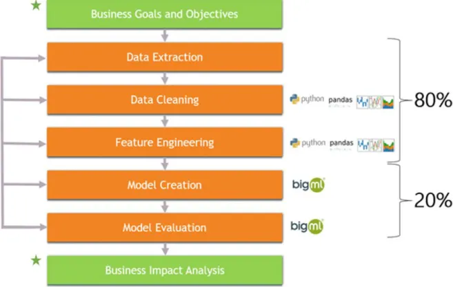
To realize a data science project there are some steps that always have to be done. This steps are the skeleton of any project. In CleverData, we always follow this procedure (Figure 2.1), and consequently, it was the one we performed in this project. Each step form part of the total project procedure, with its own characteristics and objectives.

Figure 2.1: data science project skeleton.

Each rectangle represent a step in the project. On the one hand, the steps from Data Extractionuntil Model Evaluation are related to a common data science project. Those steps are iterative between them. On the other hand, the steps with a star represent the ones that vary depending the business and its needs.

The images on the right of each rectangle are the tools used on that step. As the reader can see, the project itself didn’t need a lot of tools to be performed, that’s because the tools used are really powerful. Those tools used in project are Python [9] and the Pandas library for the steps related to data mining, and BigML [11] for the model algorithms steps.

(12)

Big numbers are time cost approximations over total time of the project. One could have a priori idea that most time spended in a project is the model creation and evaluation. However, is absolutely opposite. Data transformation process consume most time of the project. Rows are the flux between steps. This is one of the most remarkable characteristics of a data science project. Flux on traditionals projects are sequentials, there is just one iteration, however, in this type of projects, one has to work on iterations. A finished process or step can be repeated due some new condition or result.

2.1.1 Business Goals and Objectives

The base of any project are the goals and objectives that have to be achieved. This first step is really important. Decisions and strategies decided here will affect all the project itself and the direction where it will be developed .

In this step the client introduce what he wants to achieve using machine learning techniques. Then, our task is perform an analysis of those objectives in order to understand them and decide if they can be achieved using machine learning algorithms. If they can be achieved, we define how the project will be performed and which results are the one wants we want to achieve.

Sometimes, companies contact with us thinking that the issue they have can be solved using machine learning algorithms when are not. Most of the time, is caused due a general confusion about what really is machine learning and its capacities.

2.1.2 Data Extraction

Data extraction is the process of collecting all the historical data of a company. This data is considered raw due it hasn’t received any treat previously.

Data extraction is the first step that can be considered part of the data transformation process. The collection of data sometimes can be a hard work due each client has it own way to store the data. Oftenly, data is distributed among different resources and have different formats. Other times, data is poorly structured or even unstructured. All these aspects makes data extraction a hard task.

There are many tools nowadays that suits in this type of problems. Each of them has its own characteristics and methodologies, however, even with this help, the process to collect data can imply a huge work due use this tools and process are not a simple job.

(13)

2.1.3 Data Cleaning

Data cleaning is the process of detecting and removing corrupt or inaccurate records from historical data [12]. One of the most different things about a data science project done at the university and the real world is this cleaning process. Datasets used to learn and practise are most of times already clean, they don’t need to be treated.

The problem is that in real world, that’s not the case. Datasets have a lot of errors. This errors are caused from different causes and the detection of them is vital for the project. Invalid records will imply deterioration of the future model adding noise or false information.

Cleaning data is used in the process of removing data that is not relevant or needed as well. Part of the work is to know which information is relevant or can apport value to the algorithm and treat it for each specific case. Another common situation is data duplicated. Due databases are from big companies and comes from different sources sometimes the information is repeated. This provoke an overlap of information absolutely useless.

2.1.4 Feature Engineering

Feature engineering is the process of using domain knowledge of the data to create features that make machine learning algorithms work [13]. This process is fundamental in a data science project, however, is difficult and expensive. Due this high cost, most of the time of the project is spent in this task.

The task consist of finding features that add value and which ones don’t. The process encompassed creation, transformation and deletion of features, and try over all the cases the quality of the model created with those features.

Features used to train a machine learning model affect the performance of it. As better are the features, better will be the performance. The quality and quantity of features have a huge impact in the project. More than the hyperparameter configuration of the algorithm, the features are the ones that add value to the model. It is worth investing time creating new features, analysing them and transforming data than trying different algorithms. Over 80% time of the project was this step.

A complete process of generating a predicting model could be the same as the one used in a cooking recipe. Ingredients would be the data and the algorithm the recipe. If the ingredients are in poor state doesn’t matter that the recipe is the best one of the world, the food resulting

(14)

2.1.5 Model Creation

Once created the features, the machine learning model is trained. Models are feed using the data provided. Algorithm can be supervised or unsupervised and depending the objective, the project will be a classification or regression task.

In order to capt the changing behaviour of the data, those machine learning models have to be retrained periodically. This time has to be defined with the client and according to the needs of the problem.

2.1.6 Model Evaluation

The last step in the standard procedure is the model evaluation. The performance of it is the result of all the work done along the process. Depending the type of the problem there are some metrics to evaluate the performance of a model.

There are two types of evaluation, offline and online. The first one, analyse the performance of a model a priori before put it in production. The basic ways to do it is with a 80/20 split of the dataset or performing a cross-validation. The second one, test the model in current data and analyse its performance. One famous tactic used is the A/B testing. This consist of selecting a subset of instances from the total set and evaluating the results of the model to that subset.

2.1.7 Business Impact Analysis

The last step in a data science project is the impact analysis that had the solution. Companies usually trend to perform projects in order to obtain a monetary benefit. It can be directly or indirectly. On the one hand, an example of a model used to obtain a direct monetary benefit is one used for churn prediction. It give a direct income to the company due it prevents to lose clients that would churn. On the other hand, an example of a model used to obtain indirect benefits could be one that group customers based on its behaviours for a posteriori marketing strategy. This model doesn’t feedback with a direct income, however, the knowledge of the patterns of that customers can lead to future incomes.

In CleverData we can help to our client to understand what is data telling about a business, however, at the end, the client is the one who has to apply the corresponding actions.

2.2 BigML

One of the most discussed topics in the BigData and Machine Learning fields are the methods and tools used. Searching on the internet, reading articles or speaking with other companies give a huge variety of options to choose. Each method or tool has its own properties and

(15)

advantages, however, at the end, everyone has a different opinion. Each person will defend its own way to work.

This advantage of different resources can be a double-edged sword. At the moment to start a project, you can get lost over this huge world of options and get confused. My recommendation is to think twice which tool use and think about which resources you have. Spending time thinking which tool use can imply to reduce effort and time on the future. A bad selection of tools can consequence into future problems.

At CleverData our main tool used to develop data science projects is BigML. BigML is a pioneer system of machine learning as a service. Is a highly scalable, cloud based machine learning service that is easy to use, seamless to integrate and instantly actionable.

What makes BigML special is that any person, independently of the background, can use it. As Francisco J.Martín, Co-Founder and CEO of BigML said in an interview “ Es una herramienta que sirve para aprender de los datos de forma muy fácil. No hay que saber nada de data science para usar BigML. Es una cosa bastante mágica, el sistema encuentra patrones de forma automática. Nuestro objetivo es automatizar las tareas del machine learning y democratizarlo. BigML está a disposición de todo el mundo, basta con arrastrar un fichero de datos. De forma automática el sistema analiza los datos y crea un data set estructurado, después es capaz de encontrar los patrones y generar un formulario para jugar con las variables”

[14].

The service offers a wide range of different supervised and unsupervised algorithms. Moreover, it has resources that allows the user to create workflows in a easy way. The three main modes to use the service are:

● Web interface: This is the most common way to use it. Is a web user interface that is

very intuitive. This is their main strong point. Allow the user to realize all the flux of steps in a very easy way.

● Command Line Interface: A command line tool call bigmler. Permit more flexibility

than the web. I’ve never used it, I worked directly with the API.

● API: A RESTful API provided in many programing languages: Python, Java, Node.js, Clojure, Swift, Objective-C, C#, PHP.

The service can be used in development mode or production mode. The first one is free, however, the drawback is the limitation of size tasks. The second one is a paid mode, there are different plans, each one of them with its own characteristics.

(16)

options and parameters that converts it in a powerful tool. However, due it will be endless for the reader, won’t be described in detail each of its options. To go deep in details I recommend read the BigML documentation that is on the web.

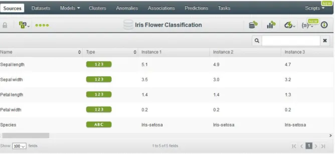
2.2.1.1 Sources

Sources are the raw data for the problem under study. BigML accept different formats file, however, the most common used is a CSV. BigML also accept as source remotes files by a specific URL or files from specific servers. Once the source is upload, there is a range of possibilities to configure it. Select the type of the features, the language of the source, missing values, how has to be treated text or item features are some of the options it has (Figures 2.2 and 2.3).

Figure 2.2: Source data.

(17)

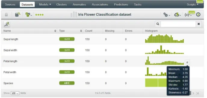
2.2.1.2 Datasets

Datasets are views of the data source that the user can use as the basis for building models. Datasets specify the target attribute (class in classification or output in regression). Each feature is summarized with a bar graph that permits its visualization (Figure 2.4). In addition, user can see some variables as mean, median, standard deviation over others that permits a first analysis of the features’ distribution.

Figure 2.4: Features distribution.

There is also a very common used training and test set split resource that separate an original dataset into a training and test dataset for a controlled evaluation of a models performance later. User can choose the proportion data of each set, however, the most common, is the typical 80-20 percent split (Figure 2.5)

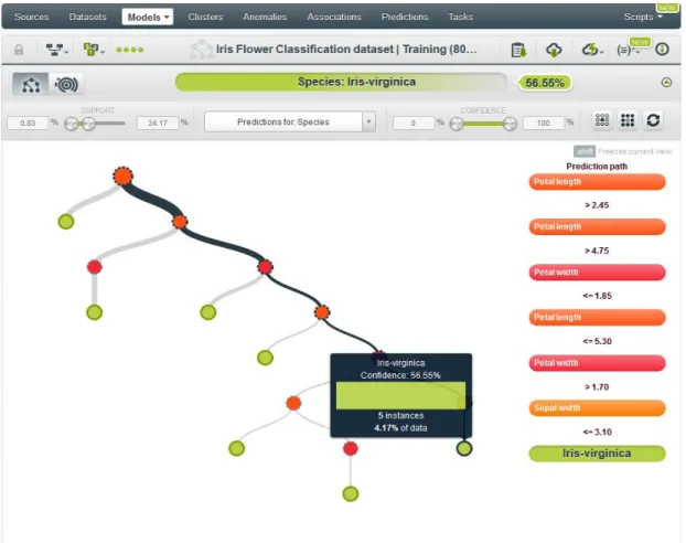
Figure 2.5: Split dataset. 2.2.1.3 Models

(18)

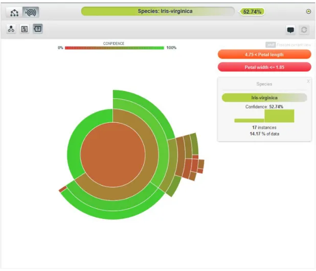
clean presentation of the model (Figure 2.6). BigML offers a sunburst view representation as well (Figure 2.7).

As in the different resources, models has its own properties that makes them flexible to the user demands. Som options as the balanced objective, or the number of leafs are examples of the variety parameters configuration.

(19)

Figure 2.7: Sunburst view.

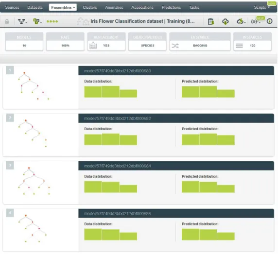
2.2.1.4 Ensembles

An ensemble is a collection of models which work together to create a stronger model with better predictive (Figure 2.8). BigML currently provides two types of ensembles:

● Bagging (a.k.a. Bootstrap Aggregating): builds each model from a random subset of

dataset. By default the samples are taken using a rate of 100% with replacement. While this is a simple strategy, it often outperforms more complex strategies.

● Random Decision Forests: similar to Bagging however, also chooses from among a

(20)

Figure 2.8: Ensemble.

Ensembles and models, once trained, have the option to visualize an ordered list with the field importance (Figure 2.9). This simple characteristic, that permits the user a first analysis, is even more useful for clients. As mentioned before, as important to understand the results, is the transmition of them to clients. Due most of time, clients wants brief and simple answers, this visualization is perfect.

(21)

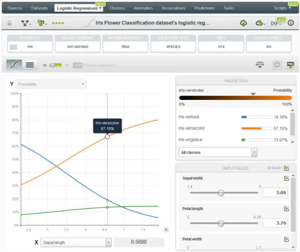
2.2.1.5 Logistic Regressions

A logistic regression is a supervised Machine Learning method to solve classification problems. For each class of the objective field, the logistic regression computes a probability modeled as a logistic function value, whose argument is a linear combination of the field values (Figure 2.10).

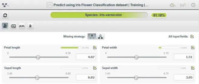
Figure 2.10: Logistic Regression. 2.2.1.6 Predictions

BigML permits predictions for single instances or for many instances in a batch (Figure 2.11). Each prediction has a categorical or numerical output depending if it is a classification or regression problem respectively. In addition, for each prediction there is its confidence or expected error respectively.

(22)

Figure 2.11: Single Prediction. 2.2.1.7 Evaluations

BigML provide an easy way to measure and compare the performance of classification and regression models. The main purpose of evaluations is twofold:

● First, obtaining an estimation of the model’s performance in production (i.e., making predictions for new instances the model has never seen before).

● Second, providing a framework to compare models built using different configurations or different algorithms to help identify the models with best predictive performance.

The basic idea behind evaluations is to take some test data different from the one used to train a model and create a prediction for every instance. Then compare the actual objective field values of the instances in the test data against the predictions and compute several performance measures based on the correct results as well as the errors made by the model.

2.2.2 Unsupervised Learning

BigML offers a variety of unsupervised learning resources as well. Due the project was developed with unsupervised learning resources, they will be more detailed than the supervised learning resources. However this resources will be deeply explained in the next section, here are just introduced.

2.2.2.1 Clusters

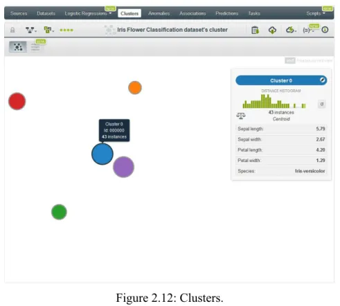
BigML Clusters provide powerful visualizations of the results of clustering data instances, which gives insight into their internal structure. In addition their visual representations, clusters also provide a textual summary view of the most essential information about them (Figure 2.12). Clusters uses proprietary unsupervised learning algorithms to group together

(23)

the instances that are closer together according to a distance measure, computed using the values of the fields as input.

Figure 2.12: Clusters.

BigML Clusters can be built using two different unsupervised learning algorithms:

● K-means: the number of centroids need to be specified in advance.

● G-means: learns the number of different clusters by iteratively taking existing cluster

groups and testing whether the cluster’s neighborhood appears Gaussian in its distribution.

Both algorithms support a number of configuration options, such as scales and weights, over others.

2.2.2.2 Anomalies

Identify instances within a dataset that do not conform to a regular pattern (Figure 2.13). BigML’s anomaly detector is an optimized implementation of the Isolation Forest algorithm, a highly scalable method that can efficiently deal with high-dimensional datasets.

(24)

Figure 2.13: Anomaly Detection. 2.2.2.3 Associations

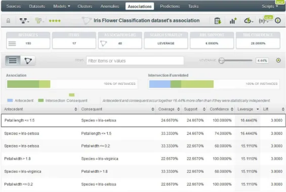
Find meaningful relationships among fields and their values in high-dimensional datasets (Figure 2.14).

(25)

2.3 Models Learning

In this project basically we used just 2 different algorithm. One for the first step of clustering, and another one for the association rules. Both algorithm are propriety of BigML. Moreover, this algorithm are modifications of the original algorithms. BigML transform them in order to improve its performance or adapt to its servers.

The algorithm used to group stores into clusters was G-means. G-means is a clustering algorithm similar to the typical K-means. The most important difference, is that in G-means the number of clusters K is not chosen, is the algorithm itself that detect the appropriate number of clusters. In our case, due the client was not looking for a specific number of clusters, he just was looking for around 9 clusters, we decided to let the algorithm chose the appropriate number of clusters, and so, use G-means.

In the association discovery step was used a BigML algorithm as well. This algorithm was acquired from Professor Geoff Webb (Monash University). With it we were able to discover the associations rules that has each cluster.

2.3.1 Clustering Models

There are problems that require separating datasets into subsets of instances bearing some similarities. Cluster analysis is a Machine Learning task that partitions a dataset and groups together those instances that are similar. It separates a set of instances into a number of groups so that instances in the same group, called cluster, are more similar to each other than to those in other groups. Cluster analysis does not require using previously labeled data. For this reason, it falls under the category of unsupervised learning.

BigML clusters use proprietary learning algorithms to group together the instances according to a distance measure, computed using the values of the fields as input. Each cluster group is represented by its center (or centroid). All BigML field types are valid inputs for clustering, i.e. categorical, numeric, text and items fields, although there are a few caveats. First, numeric fields are automatically scaled to ensure that their different magnitudes do not bias the distance calculation. Second, clustering does not tolerate missing values for numeric fields, so BigML provides several strategies for dealing with them (see Section 4.4), otherwise those instances are excluded to compute the clusters.

BigML clusters can be built using two different unsupervised learning algorithms:

(26)

● G-means: the algorithm automatically learns the number of different clusters by iteratively taking existing cluster groups and testing whether the cluster’s neighborhood appears Gaussian in its distribution.

2.3.1.1 K-means

K-means is one of two algorithms that BigML provides for cluster analysis. K-means clustering aims to partition data instances of a dataset in K clusters, such that each data instance belongs to the cluster with the nearest center.

The K-means implementation of BigML is optimized for scalability, with this is mitigated one of the major limitation of the standard K-means. BigML use the mini-batch approach [15]. This method reduce the computational cost by orders of magnitude compared to the classic K-means algorithm.

A characteristic of K-means is how the algorithm is initialized. The initialization affects the quality of the identified clusters due the centroids are randomly chosen in the beginning. This means that the quality of the clusters identified by the algorithm usually varies for each run, so it is fair to say that standard k-means provides no guarantee of accuracy [16]. Due this problem, alternative approaches for the selection of initial clusters have been studied, such as K-means++ which provide a good solution however, is a little slow for BigML purposes. Instead, BigML use the K-means|| approach, which is similar to K-means++, however, much faster.

Another key aspect where BigML clusters improve on standard K-means is the way how are handle categorical features. Instead of “binarizing” each category, meaning a field with 10 categories becomes 10 binary fields, BigML use a technique called k-prototypes which modifies the distance function to be more category-friendly so each cluster chooses the most common category from its neighborhood. So, BigML Clusters use mode instead of mean for categorical fields.

2.3.1.2 G-means

Sometimes is hard to know in advance how many clusters can be identified in a dataset or simply you don’t want to force the algorithm to output a specific number of clusters. To solve this issue, G-means [17] was created.

G-means use a special technique for running K-means multiple times while adding centroids in a hierarchal fashion. G-means has the advantage of being relatively resilient to covariance in clusters and has no need to compute a global covariance.

BigML use a different implementation than one explained in the paper. First, BigML reuse the sample-based K-means rather than running full K-means, with the already described

(27)

performance and scalability advantage. Additionally, BigML clusters choose new candidate clusters with K-means|| rather than the PCA calculation from the paper. While this gives us better scalability, it means BigML’s version of G-means is no longer deterministic as in the paper.

Finally, BigML G-means have different stopping criteria than the original paper. BigML currently enforce a maximum limit of 128 clusters. In addition, if the algorithm doesn’t make sufficient progress in finding Gaussian clusters after multiple iterations of G-means, it stops early. Both techniques ensure that the algorithm returns fewer clusters.

G-means is almost parameter-free, except for one, the critical_value parameter. G-means iteratively takes existing clusters and tests whether the cluster’s neighborhood appears Gaussian. If it doesn’t, the cluster is split into two. The critical_value sets how strict the test is when deciding whether data looks Gaussian. The current default is 5, however, ranges between 1 and 20 can be reasonable depending on the dataset. A critical value of 1 means data must look very Gaussian to pass the test and can lead to more clusters being detected. Higher critical_values will tend to find fewer clusters.

2.3.2 Association Discovery

There are problems that require to find meaningful relationships among two or more values in large datasets across thousands of values, e.g., discovering which products are buy together by customers (i.e., market basket analysis), finding interesting web usage patterns, or detecting software intrusion. These problems can be solved using Association Discovery, a well-known unsupervised learning technique to find relevant associations among values in high-dimensional datasets.

The BigML associations algorithm was acquired from Professor Geoff Webb (Monash University), a globally acknowledged expert, who spent ten years developing the association discovery in Magnum Opus.

(28)

● Avoids the problems associated with model selection. Most Machine Learning techniques produce a single global model of the data. A problem with such a strategy is that there will often be many such models, all of which describe the available data equally well. A typical model chooses between these models arbitrarily, without necessarily notifying the user that these alternatives exist. However, while the system may have no reason for preferring one model over another, the user may, e.g., two medical tests may be almost equally predictive in a given application. If so, the user is likely to prefer the model that uses the test that is cheaper or less invasive.

● A single model that is globally optimal may be locally suboptimal in specific regions of the problem space. By seeking local models, association mining can find models that are optimal in any given region. If there is no need for a global model, locally optimized models may be more effective.

Association Discovery has been extensively researched over the last two decades. It is distinguished from existing statistical techniques for categorical association analysis in three respects:

● Association Discovery techniques scale to high-dimensional data. The standard statistical approach to categorical association analysis, log-linear analysis [18] has complexity that is exponential with respect to the number of variables. In contrast, Association Discovery techniques can typically handle many thousands of variables.

● Association Discovery concentrates on discovering relationships between values rather than variables. This is a non-trivial distinction. If someone is told that there is an association between gender and some medical condition, they are likely to immediately wish to know which gender is positively associated with the condition and which is not. Association Discovery goes directly to this question of interest. Furthermore, associations between values, rather than variables, can be more powerful (i.e., discover weaker relationships) when variables have more than two values. Statistical techniques may have difficulty detecting an association when there are many values for each variable and two values are strongly associated, however, there are only weak interactions among the remaining values.

● Association Discovery focuses on finding associations that are useful for the user, whereas statistical techniques focus on controlling the risk of making false discoveries. In contexts where there are very large numbers of associations, it is critical to help users quickly identify which are the most important for their immediate applications.

Historically, the main body of Association Discovery research has concentrated on developing efficient techniques for finding frequent itemsets, and has paid little attention to

(29)

the questions of what types of association are useful to find and how those types of associations might be found. The dominant association mining paradigm, frequent association mining, has significant limitations and often discovers so many spurious associations that it is next to impossible to identify the potentially useful ones.

The filtered-top-k [19] association technique that underlies the BigML associations implementation was developed by Professor Geoff Webb. It focuses on finding the most useful associations for the user specific application. This approach has been successfully used in numerous scientific applications ranging from health data mining and cancer mortality studies to controlling robots and to improving e-learning.

2.3.2.1 Association Measures

This section details the precise formulas that are utilized to compute the BigML association measures. Given the association rule (A→C) where A is the antecedent itemset of the rule andC

is the consequent, and N is the total number of instances in the dataset, below are the

mathematical definitions for the measures [20] utilized by the BigML associations:

● Support: the proportion of instances in the dataset that contain an itemset.

upport(itemset)

S = number_numberof instances_of_totalthat_instancespossestheitem

upport Support(A )

S (A→C)= ⋃C

● Coverage: the support of the antecedent of an association rule, i.e., the portion of

instances in the dataset that contain the antecedent itemset. It measures how often a rule can be applied.

overage(A ) upport(A)

C →C =S

● Confidence(or Strength): the percentage of instances that contain the consequent and

antecedent together over the number of instances that only contain the antecedent. Confidence is computed using the support of the association rule over the coverage of the antecedent.

onfidence(A )

C →C = Support_Support(A₍→_A₎C)

(30)

● Lift: how many times more often antecedent and consequent occur together than expected if they were statistically independent.

ift(A )

(31)

3 Design and Application of Market

Basket Analysis Methodology

3.1 Project Methodology

Through previous chapters, most aspect of the project were already described. However, a brief summary of the project process will be described following to have a general view of the procedure. In addition, there are some details that has to be mentioned about the design of the project that affected its procedure.

Our objective in his project was the analysis of customers purchases and its behaviour. To do it, the project was divided in two steps. The first one, was a store clustering. Group stores based on its behaviours. The second one, was the analysis of associations rules of its items for each cluster.

The first step we realized was the problem definition. Which thing the client wanted to achieve with this project. All this step was described in the “Introduction

” chapter.

The second step was the obtention of data. Companies usually have its data in data warehouse [21] or databases [22] and the extraction of it is a difficult task that requires a huge work. In order to design a good data science project, automatic workflows of that extraction has to be done. That’s because, as it was mentioned previously, machine learning models have to be retrained periodically. However, for the first model of associations rules, the client was not interested in this automatic workflow. Due that, all the data used in this project was given in a

csv

format.

Once we obtained the data we had to clean it. Throughout the project we removed data that was incorrect or invalid. Is common that data have mistakes, is impossible to have everything in order in a company, that’s why a data cleaning task is performed. However, there are cases where some instances have to be removed although are correct because they are considered anomalies. Anomaly detection [23] is the identification of observations which do not conform to an expected pattern or other items in a dataset. This concept has not to be confused with data cleaning, due the cleaning data process search for invalid records. Anomalies detection just looks for records that not form part of a pattern. Depending the objective of the project, this anomalies can be noise or be exactly what you are looking for. For instance, in fraud detection problems, those instance that don’t conform a regular pattern

(32)

In our project, the store with id614

had2500m2when the second shop with more meters was

the 525

with 1400m2.The store 614 was so big due the client consider as a single store an

entire commercial center and rents parts of the area to different business. This traduced to patterns, means an anomaly store. Our issue was to decide if we removed this store from the clustering process. At the end, we decided to kept it due the client was interested to know in which cluster the clustering algorithm classified it. In addition, in the same process of data cleaning, we decided to remove plastics bags and parking records from the tickets historical due they didn’t add valuable information to the project.

In the clustering step we had to choose between two different clustering algorithms that BigML has, K-means and G-means. Each of them has its own characteristics. In the “Clustering Models” chapters both are described. At the beginning of the project we considered to use both algorithm and analyze its results, however, due the client didn’t have in mind a specific number of clusters to find, we used G-means in this project. The only condition was that the numbers of clusters was acceptable for its purposes. A low number of clusters will be useless for the client cause he couldn’t discover remarkable differences between stores of each cluster, and a high number of cluster would be impossible for the client to apply a specific marketing strategy for each of them. For instance, if a cluster were composed for 4 shops had no rentability study and apply a strategy just for these stores. We decided to improve the data representation until G-means algorithm output 9 clusters.

In order to evaluate the clustering models we were obtaining, we were in periodically contact with the client. In classification problems, there are many techniques to analyse the performance of a model. However, in a clustering problem, the evaluation of it is more complicate, due there is no target to predict and compare results. Thus, to evaluate our clustering model, we were in constant contact with the client presenting the results we were obtaining. Moreover, at the end of the project, we presented to the client the association rules created for each cluster.

3.2 Software & Hardware used

As BigML is the one responsible of all the machine learning algorithms all this process was done on its servers, we didn’t need hardware for it. However, for the feature engineering task, we needed it.

The software used in this project was the programming language Python. In addition, we used one of the most powerful libraries used nowadays for Data Science, Pandas. The environment to programme used was Jupyter Notebook [25].

(33)

To process all the data we used a Windows server. We upload there all the data needed and used via remote, the software previously mentioned to realize the feature engineering. Moreover, we had a personal laptop to analyse data, results and connect to BigML.

Server

● Windows Edition: Windows Server 2012 R2 Standard

● Processor: Intel(R) Xeon(R) CPU E5-2047 v2 @ 2.40GHz 2.40 GHz

● Installed memory (RAM): 24.00 GB

● System type: 64-bit Operating System, x64 based processor Laptop

● Windows Edition: Windows 10 Enterprise

● Processor: Intel(R) Core(TM) i7-5500U CPU @ 2.40GHz 2.40GHz

● Installed memory (RAM): 8.00GB

● System type: 64-bit Operating System, x64 based processor

3.3 Data

Through time, we have faced different projects on CleverData. Always that we start a new project, on the first meeting with the client, we perform the same question, which data posses. This question is maybe one of the most important ones. Depending the answer, we can know instantly if the project can be performed or not. The key in any data science project is data. Data is the principal component that makes a projects success or fail. Is the machine learning algorithms combustible. With no data, we cannot make miracles. However, if we possess the correct data, we can start to work.

One question we often listen from our clients is the quantity of data they need to start to using machine learning. They collect data like if they have diogenes syndrome. Influenced by the famous concept of Big Data. However, to use machine learning is not needed a huge amount of data. That’s one advice we repeat constantly to our clients in CleverData. More than the quantity of data, the important is the quality of it. Without quality, the algorithm cannot learn any pattern from data, there is just a lot of nonsense data and noise. For instance, we face some projects where we have a lot of data. However, when we start to look the given data trying to understand what means we discover inconsistencies on it. Maybe some variables are not well calculated or others has no sense. All this “mistakes” influence negatively the model. In our case, we found some mistakes in the data during the project, however, nothing special. In addition, with the huge amount of data the client provided us, it was not a problem remove those cases from data.

(34)

of stores. Each of this datasets has its own features and describe a part of the entire business. For both steps in this project, the clustering and the association discovering, we used this data Following will be described each dataset. For each of them will be a description. In addition, there will be a table summarizing the features the dataset had. This table is composed by 2 columns, the first one is the name of the feature, and the second one is the type it has.

3.3.1 Tickets dataset

● Number of Instances: 214,712,174

● Number of Attributes: 13

● Missing Values? Yes

● Size of Dataset: 21.4 GB

The first dataset used in this project was the historical tickets record. It was composed by 36,76,526 tickets from 203 different stores. Those tickets were expended during the last year, exactly from the June 2015 until May 2016. This is because we were interested in train our algorithms with newer data as possible.

A setback we had to face with this dataset was the size of it. The file was considerably large and the client had problem to send it to us. Normally, when we work on project at CleverData, we have problems at the moment to pass the data from the client to our servers. The are tools and methods used for this types of problems, are common in BigData companies. However in this project we didn’t need to use them. The solution was simple, split the file in twelve pieces, one for each month. With that, the client reduced its size and could send us the set of pieces via internet. Once we had collected all the different months was our work merge them in order to realize the feature engineering task.

The structure of the dataset was the following, each row corresponded to an item bought, and columns were features like the day, the store where it has bought, the ticket it belongs (Figure 3.2). For instance, using as guide the next image (Figure 3.1), we can see the ticket with code

20150601000001702000014

is composed by 4 different products, the 201054, 833950,

950025

(35)

Figure 3.1: Tickets dataset screenshot. Feature Type COD_DIA Date COD_FRANJA_HORARIA Categorical COD_PUNTO_VENTA Categorical COD_ARTICULO Categorical COD_OFERTA Categorical COD_VALOR_ANIADIDO Categorical COD_MARCA_PROP Categorical COD_TIPO_LINEA Categorical

(36)

UNIDADES Numerical

CANTIDAD Numerical

IMPORTE_TICKET Numerical

Figure 3.2: Ticket dataset features.

3.3.2 Articulos dataset

● Number of Instances: 60,587

● Size of Dataset: 65.5 MB

The second dataset used in the project was the stock of items our client has. This dataset contains information of each item like the family group it belongs, if it is ecologic, if it has gluten and so on.

We used this dataset basically for all the feature engineering and analysing of items per level. As we commented in previously, the client is interested in associations rules at family level. Due that, the features that will be created during the clustering step will try to capt as better as possible the behaviour of the shops related to that.

To avoid overextend the summary table (Figure 3.3) are merged some features into one. For instance, most of the features in the database are repeated twice, one has the code and the other the description. Other features are repeated in catalan and spanish, that for us is not needed. Due this overlap of information, here are just listed a list of features that represent the concept of the totally features.

Feature Type ARTICULO Categorical DEPARTAMENTO Categorical SECCION_VENTA Categorical VARIEDAD Categorical SUBFAMILIA Categorical FAMILIA Categorical SECCION Categorical

(37)

SECTOR Categorical ESTRUCTURA Categorical SUBCATEGORIA Categorical CATEGORIA Categorical GESTOR Categorical PLANOGRAMA Categorical MARCA_PROPIA Categorical SEG_ALFABETICA Categorical GESTION_PIEZAS_PDV Categorical TOTAL Categorical COMPRADOR Categorical AGRUPACION Categorical JEFE_AREA_COMPRAS Categorical SECTOR_NEP Categorical SECCION_NEP Categorical OFICIO_NEP Categorical CATEGORIA_NEP Categorical FAMILIA_NEP Categorical SUBFAMILIA_NEP Categorical VARIEDAD_NEP Categorical PRODUCTO_APL Categorical PRODUCTO_ECO Categorical PRODUCTO_SGLU Categorical TIPO_ALTA Categorical NUEVA_MARCA Categorical

(38)

3.3.3 Puntos Venta dataset

● Number of Instances: 273

● Size of Dataset: 226 KB

The last dataset used contains information of each store the client posses. This information belongs to structural and un-structural variables like the size of the store, the location of it or the shop category it belongs (Figure 3.4).

Our hypothesis was that shops can be similars due structural and un-structural variables. For instance, a shop with parking will have a higher mean ticket due the people go there on car and can take with him more products. Or the category of the shop can lead to have some specific products that others don’t have. All this information Influenced the behaviour of the shop.

Our client tried in past occasions classify its stores using some metrics. However, due we didn’t know how were they created or based on, we decided to not use them in the clustering to not add noising information. In addition, the client was interested to see how the algorithm classified the stores, so we didn’t use those features.

PUNTO_VENTA Categorical TIP_PUNTO_VENTA Categorical ENSENA Categorical HISTORICO Categorical REGION Categorical PROVINCIA Categorical COMARCA Categorical MUNICIPIO Categorical DISTRITO Categorical COORD_ZONA Categorical SUPERVISOR Categorical TARIFA Categorical

(39)

GAMA Categorical COMPARABLE_01 Categorical COMPARABLE_02 Categorical FECHA_APERTURA Date FECHA_CIERRE Date POSTAL Categorical EMPRESA Categorical ESTADO Categorical GRUPO_COMERCIAL Categorical GAMA_MINIMA Categorical AREA_METROPOLITANA Categorical BORRADO Categorical CLASIFICACION Categorical TARIFA_CESION Categorical PARKING Categorical GRUPO_CLIENTE Categorical TERCERO Categorical CEF Categorical COMPARABLE_CHARCUTERI A Categorical COMPARABLE_CARNE Categorical COMPARABLE_FRUTA Categorical COMPARABLE_PESCADO Categorical COMPARABLE_PANADERIA Categorical MOSTRADOR_CHARCUTERIA Categorical

(40)

MOSTRADOR_PESCADO Categorical MOSTRADOR_PANADERIA Categorical FEC_ENSENA Date TALLA_CENTRO Categorical CIERRA_MEDIODIA Categorical METROS_CUADRADOS Numerical

Figure 3.4: Puntos venta dataset features.

3.4 Application of the Methodology

3.4.1 Clustering

Once we analyzed and understood the different data the client provided us, we started to work on the first part of the project, the shop clustering. Our objective was to group similar shops. The reason of this clustering was explained in a previous section.

Through this section, some of the most remarkable versions obtained during the clustering process will be described. Due during the clustering process, a large proportion of versions were created applying just little changes, not all the different versions there will be described, just the ones most remarkable or interesting. For instance, when feature is transformed into another one to add more description to the data, we create a new clustering to check how this change has affected. This little changes may or not apport significant relevance, however, they must to be checked in order to understand how the clusters evolve. This cumulative work is the reason that most part of the project is the feature engineering, because this little work, add more and more time to the project. However, at the end, the sum of all this little steps are the ones that become to successful project.

Another point to have in mind, is that the following versions were constructed based on the idea to capture the temporality of the season. Our hypothesis was that customer behaviour change through the year. In order to capture this change, we created the datasets with some features that were repeated for each trimester. Due the historical of tickets starts from June 2015 until May 2016, we decided to create the trimesters according to these groups of 4 months: {June 2015, July 2015, August 2015}, {September 2015, October 2015, November 2015}, {December 2016, January 2016, February 2016}, {March 2016, April 2016, May 2016}. This features created for each trimester can be easily identified by a“Trimestre X”

at

the end of the name,

(41)

Moreover, those stores that were opened throughout the period were excluded due we haven’t all the information. Those stores that closed throughout the period were removed as well. In the process of creation the different versions we ended up with 2 different components, a dataset and the clusters achieved with that dataset. On the one hand, the dataset is formed by instances and its features. Instances are every store of the company, and features are its information obtained from the data the client provided us. On the other hand, the clusters are the output of the clustering algorithm trained by the dataset. This clustering is created with the G-means algorithm with a critical value of 5 for all the different versions.

During the analysis of each version, there will be a description of each feature used. Some of the features are simply obtained from the original data the client provided us, others are created during the feature engineering process. Moreover, those features that need a deeper description to understand its function will be described at more detail. Due some features can be used in various versions, the description of them will not be repeated, just the new features used in the version will be described. One last thing to comment is that first feature always will be the shop id. This feature is not by the algorithm, is just an informative feature to know which shop correspond to each instance.

The structure of this descriptions will be first, the range of features that form part of that description. And then, the description itself. With this structure, we try to make, as much easy as possible, the lector reading.

3.4.1.1 Version 1

This is the first version of clustering after the decision to create features capturing the season behaviour. Some of the features are simply obtained from the original data the client provided us, others are created in the feature engineering process.

The most interesting features in this version are the ones that describe the distribution of items sold for each section. This features are the ones in the range [27-53]

. With this, we

wanted to add more information about the items sold. This concept of items sold for each category has a name in the market analysis, the market share.

Market share [26] is the percentage of an industry or market's total sales that is earned by a particular company over a specified time period. Market share is calculated by taking the company's sales over the period and dividing it by the total sales of the industry over the same period. This metric is used to give a general idea of the size of a company in relation to its market and its competitors.

(42)

Features [1]:

Id of the shop.

Features [2]:

Price of the most expensive ticket.

Features [3]:

Mean price of all tickets.

Features [4-6]:

Mean units sold per day, week and month.

Features [7-13]: Which percent of items from total are sold on each week day. The sum of all this values up to 100.

Features [14]:

Number of items sold from the client’s brand.

Features [15]:

Number of items sold from others brands.

Features [16]:

Number of different items the shop has.

Features [17]: Relation between the number of items sold from the client’s brand vs the number of items sold from others brand.

Features [18]:

Relation between number of items sold.

Features [19]:

Mean number of items sold per ticket. Mean number of references per ticket.

Features [20]:

Mean number of references per ticket.

Features [21-23]: The first item appears most times in tickets, the second one, and the third one.

Features [21-26]:

The first item most sold, the second one, and the third one.

Features [27-53]: Which percent of items from total are sold from each section. The sum of all this values up to 100.

Features [54-58]:

The shops posses the corresponding counter.

Feature [59]:

Segmentation the client created to classify its shops according some criterias.

Feature [60]:

Segmentation the client created to classify its shops by its size.

Feature [61]:

The shop close at midday.

Features [62-65]:

(43)

Feature [66]:

Shop’sm2

List of features used:

1. Tenda:

Id of the shop.

2. Max Ticket - Trimestre X 3. Mean Ticket - Trimestre X

4. Numero medio unidades diarios - Trimestre X 5. Numero medio unidades semanales - Trimestre X 6. Numero medio unidades mensuales - Trimestre X 7. % Unidades del total es venen en Dilluns - Trimestre X 8. % Unidades del total es venen en Dimarts - Trimestre X 9. % Unidades del total es venen en Dimecres - Trimestre X 10. % Unidades del total es venen en Dijous - Trimestre X 11. % Unidades del total es venen en Divendres - Trimestre X 12. % Unidades del total es venen en Dissabte - Trimestre X 13. % Unidades del total es venen en Diumenge - Trimestre X 14. Unidades venuts marca client- Trimestre X

15. Unidades venuts marca propia - Trimestre X 16. Numero referencias - Trimestre X

17. Relacio unidades client vs No client- Trimestre X

18. Relacio unidades venuts vs numero referencies - Trimestre X 19. Numero medio unidades por ticket - Trimestre X

20. Numero medio referencias por ticket - Trimestre X 21. TOP 1 Referencia aparece en mas tickets - Trimestre X 22. TOP 2 Referencia aparece en mas tickets - Trimestre X 23. TOP 3 Referencia aparece en mas tickets - Trimestre X 24. TOP 1 Referencia se venden mas unidades - Trimestre X 25. TOP 2 Referencia se venden mas unidades - Trimestre X 26. TOP 3 Referencia se venden mas unidades - Trimestre X 27. % ALIMENTACIO SECA sobre total ventas - Trimestre X 28. % FLECA I PASTISSERIA sobre total ventas - Trimestre X 29. % FORMATGES sobre total ventas - Trimestre X

30. % CONSERVES sobre total ventas - Trimestre X 31. % DERIVATS LACTIS sobre total ventas - Trimestre X

32. % XARCUTERIA TRADICIONAL sobre total ventas - Trimestre X 33. % PEIXOS I MARISC sobre total ventas - Trimestre X

(44)

37. % LLETS I BATUTS sobre total ventas - Trimestre X 38. % DROGUERIA sobre total ventas - Trimestre X

39. % MATERIAL TENDES sobre total ventas - Trimestre X 40. % BASSAR sobre total ventas - Trimestre X

41. % ARTICLES PUBLICITARIS sobre total ventas - Trimestre X 42. % PERFUMERIA sobre total ventas - Trimestre X

43. % PLATS CUINATS/REFRIGERATS sobre total ventas - Trimestre X 44. % CONGELATS sobre total ventas - Trimestre X

45. % Altres seccions sobre total ventas - Trimestre X

46. % FRUITES I HORTALICES sobre total ventas - Trimestre X 47. % UNITAT CARNICA sobre total ventas - Trimestre X

48. % ARTICLES TRADE MARKETING sobre total ventas - Trimestre X 49. % VENDES SENSE SECCIO sobre total ventas - Trimestre X

50. % CARBURANTS sobre total ventas - Trimestre X

51. % FUNGIBLES INF. DISKETTES sobre total ventas - Trimestre X 52. % GANGAS sobre total ventas - Trimestre X

53. % FUNGIBLES INF. DISKETTES sobre total ventas - Trimestre X 54. CHARCUTERIA 55. CARNE 56. FRUTA 57. PESCADO 58. PANADERIA 59. Tipo tienda

60. Client Talla centro 61. Cierra mediodia 62. Region 63. Provincia 64. Municipio 65. Codi postal 66. Metros cuadrados 3.4.1.2 Version 2

This is the second version of the clustering process. In this version we changed the features used for the market share and added new features to apport more information about stores’ revenue. Our hypothesis was that revenue could be a good indicator about stores behaviour, so we started to design possible features that could capture this information.

In order to capture the stores’ revenue a new feature was created, “Items 80/20”.

Based in the

Pareto principle [27], we created this feature. It was the list of the items that apported most revenue to the store. This principle is commonly used in business world. In the context of a retail business means that just a short list of differents items apport most of the revenue. For