Urban accounting and welfare indonesia

(1)

NBER WORKING PAPER SERIES

URBAN ACCOUNTING AND WELFARE

Klaus Desmet

Esteban Rossi-Hansberg

Working Paper 16615

http://www.nber.org/papers/w16615

NATIONAL BUREAU OF ECONOMIC RESEARCH

1050 Massachusetts Avenue

Cambridge, MA 02138

December 2010

We thank Kristian Behrens, Gilles Duranton, Wolfgang Keller, and Stephen Redding for helpful comments,

and Joseph Gomes and Xuexin Wang for excellent assistance with the data. We acknowledge the financial

support of the International Growth Centre at LSE (Grant RA-2009-11-015), the Comunidad de Madrid

(PROCIUDAD-CM), the Spanish Ministry of Science (ECO2008-01300) and the Excellence Program

of the Bank of Spain. The views expressed herein are those of the authors and do not necessarily reflect

the views of the National Bureau of Economic Research.

NBER working papers are circulated for discussion and comment purposes. They have not been

peer-reviewed or been subject to the review by the NBER Board of Directors that accompanies official

NBER publications.

(2)

Urban Accounting and Welfare

Klaus Desmet and Esteban Rossi-Hansberg

NBER Working Paper No. 16615

December 2010

JEL No. E1,R0,R11,R12,R13

ABSTRACT

This paper proposes a simple theory of a system of cities that decomposes the determinants of the

city size distribution into three main components: efficiency, amenities, and frictions. Higher efficiency

and better amenities lead to larger cities, but also to greater frictions through congestion and other

negative effects of agglomeration. Using data on MSAs in the United States, we parametrize the model

and empirically estimate efficiency, amenities and frictions. Counterfactual exercises show that all

three characteristics are important in that eliminating any of them leads to large population reallocations,

though the welfare effects from these reallocations are small. Overall, we find that the gains from worker

mobility across cities are modest. When allowing for externalities, we find an important city selection

effect: eliminating differences in any of the city characteristics causes many cities to exit. We apply

the same methodology to Chinese cities and find welfare effects that are many times larger than in

the U.S.

Klaus Desmet

Department of Economics

Universidad Carlos III

28903 Getafe (Madrid)

SPAIN

klaus.desmet@uc3m.es

Esteban Rossi-Hansberg

Princeton University

Department of Economics

Fisher Hall

Princeton, NJ 08544-1021

and NBER

(3)

Urban Accounting and Welfare

Klaus Desmet

Universidad Carlos III

Esteban Rossi-Hansberg

Princeton University

December 7, 2010

Abstract

This paper proposes a simple theory of a system of cities that decomposes the determinants of the city size distribution into three main components: e¢ciency, amenities, and frictions. Higher e¢ciency and better amenities lead to larger cities, but also to greater frictions through congestion and other negative e¤ects of agglomeration. Using data on MSAs in the United States, we parametrize the model and empirically estimate e¢ciency, amenities and frictions. Counterfactual exercises show that all three characteristics are important in that eliminating any of them leads to large population reallocations, though the welfare e¤ects from these re-allocations are small. Overall, we …nd that the gains from worker mobility across cities are modest. When allowing for externalities, we …nd an important city selection e¤ect: eliminating di¤erences in any of the city characteristics causes many cities to exit. We apply the same methodology to Chinese cities and …nd welfare e¤ects that are many times larger than in the U.S.

1. INTRODUCTION

(4)

that determine city sizes is crucial for answering a broad set of questions. What is the relative importance of these forces in determining the size distribution of cities? How much would we gain or lose if cities had similar amenities, technology levels or frictions? How much reallocation would this cause? How do externalities interact with these forces to determine city selection?

In this paper we provide a simple way of decomposing the characteristics that lead to the size distribution of cities into three main components: e¢ciency, amenities, and excessive frictions. We use a simple urban theory to calculate these components and to do a wide set of counterfactual exercises that provide answers to the questions we asked above. The theory consists of a multi-city model with monocentric cities that produce a single good. Workers decide how much to work and where to live. E¢ciency is modeled as TFP di¤erences, amenities as preference shocks, and excessive frictions as the cost of providing urban infrastructure that is paid for with labor taxes. To measure “excessive frictions”, we use the concept of a “labor wedge” and decompose it into the standard cost e¤ect of city size and the “excessive cost” of providing city services (see Chari, et al., 2007). We solve the general equilibrium model with and without externalities.

We use an empirical strategy to parametrize the model and to obtain the “excessive frictions” shocks and the e¢ciency shocks. We then use the model to determine the amenity shocks that make cities be of their actual sizes. The model therefore matches by construction the size distribution of cities in the U.S. The counterfactual exercises then allow us to analyze the e¤ects of the di¤erent parameter values and of the di¤erent city characteristics. For many counterfactuals we …nd that the changes in utility (and in consumption) are modest in spite of massive population reallocations. For example, eliminating e¢ciency di¤erences across cities lowers equilibrium utility levels by a mere 2.5%, and eliminating amenity di¤erences reduces welfare by just 2.3%. When we account for externalities, these numbers decline even further. The welfare implications of redistributing agents across cities due to switching o¤ any of the fundamental characteristics that account for the actual size distribution is never greater than a few percentage points.1 _{This is surprising given that the}

di¤erences in amenities and e¢ciency levels can be rather large and given that the implied population reallocations can be as large as 50%. Adding externalities has an important e¤ect on the extensive margin in the counterfactual exercises, with many cities exiting and the urban population settling in the surviving cities. However, these externalities have only modest e¤ects on welfare.

A relevant question is whether the small welfare e¤ects we uncover are inherent to the model or

1_{This resembles the literature on business cycle accounting that found that eliminating business cycles would lead}

(5)

speci…c to the U.S. To address this issue, we explore the same type of counterfactual exercises for the size distribution of cities in China. We …nd welfare e¤ects that are an order of magnitude larger than in the U.S. For example, when eliminating e¢ciency di¤erences across Chinese cities, welfare increases by 47%, compared to a corresponding 2.5% in the U.S.

(6)

amenities and excessive frictions. The model is also ‡exible enough to incorporate externalities in e¢ciency levels and amenities. With the urban characteristics in hand we can perform a variety of counterfactual exercises and calculate the welfare implications of eliminating variation in any of these characteristics. Furthermore, the proposed methodology can be used to compare urban systems across countries, although we leave that for future research.

The rest of the paper is organized as follows. Section 2 introduces a simple urban model and explains the basic urban accounting exercise. Section 3 estimates a log-linear version of the structural equations using U.S. data between 2005 and 2008 and obtains the reduced form e¤ects of the three main characteristics of cities on rents and city sizes. Section 4 performs counterfactual exercises using the empirical values of these city characteristics. Section 5 studies the e¤ect of e¢ciency and amenity shocks. Section 6 applies our methodology to China, and Section 7 concludes. Appendix A shows how the population sizes of individual cities are a¤ected when certain characteristics change. Appendix B describes in detail the urban data set constructed.

2. THE MODEL

We use a standard urban model with elastic labor supply so that labor taxes create distortions. Agents work in cities with idiosyncratic productivities and amenities. They live in mono-centric cities that require commuting infrastructures that city governments provide by levying labor taxes. Large cities are more expensive to live in because of higher labor taxes and commuting costs, but are large because of high levels of e¢ciency or local amenities. City governments can be more or less e¢cient in the provision of the public infrastructure. We refer to this variation as a city’s “excessive frictions”. In later sections we augment the model to include local externalities in production and amenities.

2.1 Technology

Consider a model of a system of cities in an economy withNtworkers. Goods are produced inI

mono-centric circular cities. Cities have a local level of productivity. Production in a cityiin period

tis given by

(7)

where Ait denotes city productivity, Kit denotes total capital and Hit total hours worked in the city.2 _{We denote the population size of city} _i _by _Nit_{. The standard …rst order conditions of this}

problem are

where small-cap letters denote per capita variables (e.g. yit=Yit=Nit). Note that capital is freely mobile across locations so there is a national interest ratert. Mobility patterns will not be determined solely by the wage,wit, so there may be equilibrium di¤erences in wages across cities at any point in time.

We can then write down the “e¢ciency wedge” which is identical to the level of productivity,Ait;

as

Agents order consumption and hour sequences according to the following utility function

1

X

t=0

t_[log_cit₊ _{log (1} _hit_{) +} i]

where _i is a city-speci…c amenity and is a parameter that governs the relative preference for leisure. Each agent lives on one unit of land and commutes from his home to work. Commuting is costly in terms of goods.

The problem of an agent in cityi0 with capitalk0 is therefore

max

2_{It would be straightforward to generalize this model to include human capital. We experimented with this, and}

(8)

where xit is investment, it is a labor tax or friction associated with the cost of building the

com-muting infrastructure,Ritare land rents andTitcommuting costs (as we will see below,Rit+Titis constant in the city so the location of the agent’s home does not a¤ect his choices).3

Throughout the paper we assume that we are in steady state so kit+1 = kit and xit = kit. Furthermore, we assumekit is such thatrt= (capital is at its Golden Rule level). The simpli…ed budget constraint of the agent becomes

cit=withit(1 it) Rit Tit: (3)

The …rst order conditions of this problem are given by1=cit= it, and

1

1 ht =wit(1 it) it;

which imply

cit

1 hit = (1 it)wit: (4)

Combining equations (1) and (4) we obtain

(1 it) =

(1 )

cit

1 hit

hit

yit: (5)

Agents can move freely across cities so utility in each period has to be determined by

u= logcit+ log (1 hit) + i; (6)

for all cities withNit>0, whereuis the economy-wide per period utility of living in a city.

2.3 Commuting Costs, Land Rents and City Equilibrium

Cities are mono-centric, all production happens at the center, and people live in surrounding areas characterized by their distance to the center, d. Cities are surrounded by a vast amount of agricultural land that can be freely converted into urban land. We normalize the price of agricultural land to zero. Since land rents are continuous in equilibrium (otherwise there would be arbitrage opportunities), this implies that at the boundary of a city, d, land rents should be zero as well, namely,R d = 0. Since all agents in a city are identical, in equilibrium they must be indi¤erent between where they live in the city, which implies that the total cost of rent plus commuting costs should be identical in all areas of the city. So

Rit(d) +T(d) =T dit = dit

3_{Since agents can move across cities, the subscript}_i_{depends on}_{t, as written under the maximization sign. To}

(9)

sinceT(d) = dwhere denotes commuting costs per mile.

we know that

Rit(d) +T(d) = Nit

1 2

alld:

This implies that

Rit(d) = dit d

and so total land rents in a city of sizeNitare given by

T Rit=

Hence, average land rents are equal to

ARit=2

Taking logs and rearranging terms, we obtain that

ln (Nit) =o1+ 2 lnARit; (7)

whereo1 is a constant.

We can also compute the total miles traveled by commuters in the city, which is given by

T Cit=

2.4 Government Budget Constraint

The government levies a labor tax, it, to pay for the transportation infrastructure. This tax can

also be interpreted as a distortion in the labor market because of the congestion created in a large city. As in Chari et al. (2007), we will refer to itas the “labor wedge”. Let government expenditure

be a function of total commuting costs and wages such that

G(hitwit; T Cit) =githitwit T Cit=githitwit 2

wheregitis a measure of government ine¢ciency. That is, the government requires gitworkers per mile commuted to build and maintain urban infrastructure. The government budget constraint is then given by

ithitNitwit=githitwit 2

(10)

which implies that the “labor wedge” can be written as

The consumer budget constraint is given by

cit=withit(1 it) Rit Tit= (1 ) (1 it)yit

Nit

1 2

:

From (5) we know that

(1 it) =

To determine output we know that the production function is given by yit =Aitkith1it and the

decision of …rms to rent capital implies thatrtkit= yit:Hence,

(11)

The free mobility assumption in (6) implies that u = logcit+ log (1 hit) + it for some ut

determined in general equilibrium so

ut+ (1 + ) log (1 + ) log (11)

The last equation determines the size of the cityNit as an implicit function of city productivity,

Ait, city amenities, _i, government ine¢ciency git;and economy-wide variables like rt andut. We can use this equation to derive the e¤ect of the three city speci…c characteristics (Ait; _it; git) on

Nit. First note that the LHS of (11) is decreasing in Nit. The LHS is also increasing inAitand i

and decreasing ingit. Hence, we can prove immediately that

dNit

So population increases in a more productive city or a city with more amenities, but it decreases in a city with a less e¢cient government.

The economy-wide utility levelut is determined by the labor market clearing condition

I

X

i=1

Nit=Nt: (13)

(12)

3. EVIDENCE OF EFFICIENCY, AMENITIES AND FRICTIONS

To lend validity to our theoretical model, we estimate the size of the three derivatives in (12) and estimate the e¤ect of land rents on population as in (7). When doing so, the general equilibrium nature of the model will be key.

3.1 Empirical Approach

We …rst estimate the “labor wedge” using equation (5) and the “e¢ciency wedge” in equation (2). Note that the empirical measure of the “e¢ciency wedge” is related not just to productivity, but also to the relative price of city output. Although we have no way of disentangling these two terms, in a theory with multiple goods relative price e¤ects across cities would have isomorphic e¤ects to changes in productivity. Hence, we just equate productivity to our measure of the “e¢ciency wedge”.

The general equilibrium nature of the model is important. For example, if we regress the log of city size on the log of the labor wedge, we …nd a statistically signi…cant positive e¤ect (coe¢cient of 1.2360 and p-value of 0.000). But it would be wrong to conclude from there that higher frictions lead to greater city size. Rather, according to the theory, this positive association would re‡ect more productive cities being larger, and larger cities experiencing greater commuting costs. That is, in as far as greater commuting costs are due to cities being more e¢cient, they will be positively associated with city size. Only frictions “in excess” of this basic tradeo¤ between e¢ciency and congestion will have a negative e¤ect on city size. In what follows we propose a methodology that accounts for these general equilibrium links by decomposing these di¤erent e¤ects.

We start by estimating the following equation

lnNit= 1+ 1lnAit+"1it: (14)

The value of 1 yields the e¤ect of the “e¢ciency wedge” on city population. According to the

model, 1>0 by (12). Furthermore,ln ~Nit(Ait) = 1lnAit is the population size explained by the

size of the “e¢ciency wedge”. In contrast, "1it is the part of the observed population in the city that is unrelated to productivity; according to the model it is related to both git and _it. We can thus de…ne the function~"1(git; it) "1it.

(13)

and agglomeration. We can estimate the e¤ect of productivity on the “labor wedge” by using equation (10) and the decomposition of lnNit intoln ~Nit(Ait)and "1it provided by equation (14). Hence, we estimate

ln it= 2+ 2ln ~Nit(Ait) +"2it: (15)

According to equation (10), 2 > 0. That is, a city that is more productive and so has more

population, will be more distorted. We denote the e¤ect of e¢ciency on distortions by lnfit = 2ln ~Nit(Ait). Equation (10) also implies that the error term"2itis related togitand to~"1(git; it)

(since the labor wedge depends on all factors a¤ecting population and not just on ln ~Nit(Ait)). Hence, we de…ne~"2(git;~"1(git; _it)) "2it.

We now use equation (7) to decompose the e¤ect from all three elements of(Ait; _i; git). To do so, we estimate

ln (ARit) = 3+ 3lnfit+ 4"1it+ 5"2it+"3it (16)

using median rents forARit: The model has clear predictions for 3, 4 and 5. In particular, it

implies 3>0, since by equations (7) and (12) e¢ciency has a positive e¤ect on population, which

has a positive e¤ect on the level of distortions and on average rents. This is the standard city size e¤ect. The e¤ects of _it and git are determined by the estimates of 4 and 5. Note that "1it

and"2it depend on both _itand git. However, since "2it= ~"2(git;~"1(git; _it))depends only on _it through "1it and we are including "1it directly in the regression, 5 will capture only the e¤ect of

changes in git on land rents. So, 5 captures the e¤ect of git on frictions and therefore average

rents. Higher distortions imply a higher it. Hence, the model implies that highergit, and therefore

higher itand"2it, implies lower population and lower rents (see (12)). Thus 5should be negative.

Similarly, since we are controlling for the e¤ect ofgit by including"2it, 4 will capture the e¤ect of "1iton land rents controlling forgit, which is the e¤ect of it on land rents, since"1it= ~"1(git; it):

Hence, the model implies that 4 should be positive by equations (7) and (12). Our model implies

that rents are a non-linear function of (Ait; i; git). In contrast, equation (16) assumes that it is

a linear function. Adding higher degree polynomials and interaction terms to this relationship can in principle be important. We do so in our empirical implementation below, though this does not a¤ect results in any substantial way.

Note that we can then use equation (7) to relate average rents and population sizes. So we estimate equation (7) as

(14)

According to the model, in a circular city, 6= 2>0.

3.2 E¤ects of E¢ciency, Amenities and Frictions on City Size

To bring the model to the data, we construct a new data set on U.S. metropolitan statistical areas (MSAs) for the period 2005-2008. Apart from output and rental prices, few ready-to-use data are available at the MSA level. We rely on a combination of proxies previously used in the literature and micro-data to come up with measures for the other relevant variables, such as consumption, hours worked, and capital. Appendix B.1 provides details on the construction of the data set. Computing the “labor wedge” and the “e¢ciency wedge” requires making assumptions on the values of some parameter values. Table 1 reports the parameter values we use and provides brief comments on the chosen values. Essentially, they make the model match key moments in the aggregate.

To implement the empirical exercise of the previous section, we pool the data for 2005-2008, and include time dummies in all regressions. One further di¤erence is that we also include an interaction term"1it"2itin equation (16), since we found it to be statistically highly signi…cant. We denote the coe¢cient associated with this interaction term 7. Standard errors for equations (16) and (15) are

obtained by bootstrapping, since some of the regressors are estimated.4 _{The results are presented}

in Table 2.

Table 1 Parameter Value Comments

1:4841 McGrattan and Prescott (2009)

0:3358 McGrattan and Prescott (2009)

r 0:02 Standard number in the literature

0:02 Theory requires =r

As is clear from Table 2, all coe¢cients have the signs implied by the model and are highly signi…cant. The estimation of equations (14), (15), (16), and (17) yield R2 _{values of, respectively,}

0:14,0:37,0:25,0:18. The model implies that in a circular city 6= 2. The value we …nd is close to

two and we fail to reject the hypothesis that it is equal to two a the 5% level.

4_{Correcting the standard errors for clustering by MSA does not qualitatively change any of the results, except for}

(15)

Table 2

j j s.e. p-value Theoretical Prediction

1 2:0964 0:3727 0:000 +

2 0:4127 0:0234 0:000 +

3 0:1283 0:0461 0:005 +

4 0:0959 0:0070 0:000 +

5 0:2020 0:0420 0:000

6 2:1400 0:1652 0:000 2

7 0:1841 0:0437 0:000

Number of observations: 768

These results allow us to reach several conclusions. First, highly e¢cient cities are more populated. This is consistent with numerous empirical studies in the literature. Second, e¢cient cities are more distorted. Frictions are larger as a result of these cities being larger. The frictions that result from more e¢cient cities being larger are positively related to median rents as they are the result of the higher e¢ciency. Third, frictions that exceed the ones explained by e¢ciency have a negative e¤ect on land rents and city size. Finally, cities that are larger due to amenities also exhibit larger median rents.

(16)

4. COUNTERFACTUAL EXERCISES

4.1 Methodology and Shock Identi…cation

The model provides a straightforward way of performing counterfactual exercises. Equation (11) implies that

Ifgit and are small using the approximationlog (1 x) x;5 _{we obtain}

Nit= ₂

This solvesNitas a function of(Ait; it; git). Note that the approximation results in exactly the same

derivatives with respect to(Ait; it; git). Furthermore, @Nit=@u <0; namely, a higher equilibrium

utility (smaller total population) makes concentration of workers in a given city less likely since concentration implies congestion costs.6

We can use the equation above to calculate Nitgiven the values of (Ait; it; git)and other

para-meter values. We can also use these expressions to run counterfactual exercises. In particular we can calculate counterfactual distributions of city sizes assuming that all cities have similar values of

5_{This approximation works best if}

itand are small. In the exercise below the approximation error is likely very

small.

6_{Throughout this section we calculate an agents’ utility based on his labor and capital income but not the income}

that agents obtain from land rents. Land is owned by absentee landlords and so rental income does not enter an agent’s utility and does not a¤ect their decision to move. We have calculated all of the results below if we use the alternative assumption that workers in a city own a diversi…ed portfolio of land in the city and so obtain as income the average rents. The results under this assumption are essentially identical (utility di¤ers only by less than 0.001) to the ones with absentee landlords, both in the case with and without externalities. The reason is that we are always

normalizing the level of utility that reproduces the size distribution tou= 10 and only relative utilities matter to

(17)

any of the exogenous city characteristics(Ait; it; git). Note thatuthas to be selected such that the

resulting city sizes satisfy the labor market clearing condition (13).

In order to perform any of these exercises we …rst need to develop a strategy to calculate

(Ait; it; git)for each city. Aitcan be calculated directly from available data since Ait= yit

k_ith1_it

and we have data onyit,hitandkit:This is what we did in the empirical implementation above. An alternative way of calculating the relevant productivity and skill term without using kit (which is potentially poorly measured in the data) is to use the prediction of the model on capital allocation. In particular the model implies thatrtkit= yitand so

kit= yit

rt :

We can then let

Ait= y

1 it

rt h

1 it

:

Equation (18) assumes that capital is determined in this way and so this method has the advantage of being theoretically more consistent (although it does not use the actual data on capital stocks). We have added capital in both ways, and found the results to be similar. The correlation of the model-based capital stock measure and the empirical capital stock measure is 0.9. Therefore, we omit here the exercise with the theoretical levels of capital and focus on the one where we use the empirical measure of the capital stock. (Figure A9 in the appendix shows the results when we use theory-based capital levels).

Obtaining values for the other two city characteristics is more complicated. First note that equation (10) can be used to estimategit. Based on this equation we can run the simple log-linear regression

ln it= 5+ 8lnNit+"5it: (19)

Equation (10) then implies that"5it= lngit. Using data for 2005-2008 and adding time dummies, we estimate 8= 0:08 with a standard error of0:009. TheR2 of the regression is 0:10. Note that

equation (10) implies that 8 = 0:5, so the estimated coe¢cient is signi…cantly lower than the one

(18)

8= 0:5 . Independently of how the coe¢cient 8maps with the theory, the equation allows us

to recover the frictions not associated to population size, which constitute the natural logarithm of the city’s “excessive frictions”.

We still have to obtain the value of it. There are a variety of ways to do this. The one that

is most consistent with the theory is to use equation (18) and solve for the set of it that make

the model match city sizes exactly, given some normalization of u(we set u= 10). We can then …x _it and perform counterfactual exercises. Of course, this exercise depends on the value of all parameters in the model. As before, we use the parameters in Table 1, which match key moments in the aggregate. One important parameter in determining _it is , for which we have not assigned a value yet. To obtain a value for we also use equation (19) that regresses the labor wedge on city population size. In discussing the results of estimating this equation, we already pointed out that the theoretical value of the coe¢cient on population size ( 8) should be 0.5 according to the theory.

So we …x it at this value and estimate the constant 5. Furthermore, equation (9) then implies that

5= ln 2

3 + ln

1 2ln

and so, given a value for 5, we can calculate . The estimation yields a constant equal to 7:3179,

which yields a value of = 0:00176. The time dummies we include are mostly not signi…cant, but adding their values would yield a constant that is somewhat smaller which would imply a lower . Therefore, we use a value of = 0:001and do many robustness checks for higher values of .

4.2 Counterfactuals

(19)

4 6 8 10 12 14 16 18 -6

-5 -4 -3 -2 -1 0

ln(population)

ln(prob>population)

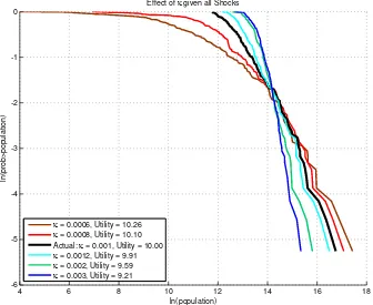
Effect of  given all Shocks

 = 0.0006, Utility = 10.26

 = 0.0008, Utility = 10.10 Actual:  = 0.001, Utility = 10.00

 = 0.0012, Utility = 9.91

 = 0.002, Utility = 9.59

 = 0.003, Utility = 9.21

Figure 1: The City Size Distribution for Di¤erent Levels of Commuting Costs

Figure 1 shows the actual distribution of city sizes in the U.S. and counterfactual distributions of city sizes if we increase or decrease commuting costs , given the distribution of characteristics. The results are presented in the standard log population – log rank plots in which a Pareto distribution would be depicted as a line with slope equal to minus the Pareto coe¢cient. As is well known, the actual distribution is close to a Pareto distribution with coe¢cient one. By construction the model matches the actual distribution exactly for = 0:001. In that case we normalize utility u= 10:7

In all counterfactual exercises we solve for the value of u for which the labor market clears, i.e., the sum of population across cities equals the actual total urban population. Note that percentage changes in utility are equivalent to percentage changes in consumption since we are using a log-utility speci…cation. Figure 1 shows that larger commuting costs make the largest cities smaller

7_{This normalization a¤ects the size of the welfare changes due to the level taken by the amenity characteristics.}

On average we …nd that the share of utility coming from amenities is around 28%. We have no evidence that this number is reasonable. However, it is easy to adjust the numbers to be consistent with any share of amenities in utility. For example, if the share of utility coming from amenities is set to zero, all our utility numbers from counterfactuals

(20)

and the smaller cities larger, leading to a less dispersed distribution of city sizes. The 20% increase in commuting costs decreases utility by about 0.9%. The decline in commuting costs increases dispersion and raises utility by 1%. Note that the smallest cities now become much smaller. The main advantage of some of these cities was their small size and their low commuting costs. As commuting costs decrease, this advantage becomes less important and their size decreases further. If we double or triple to 0.002 and 0.003 we obtain changes in utility of around 4% and 8%. Large cities now become much smaller, which implies that production is not done in the most productive and highest amenity cities which leads to substantial welfare losses.

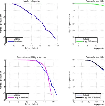
11 12 13 14 15 16 17

ln(prob > population)

Model Utility = 10

Counterfactual Utility = 10.2497

Actual

Avg. Exc. Frictions

(21)

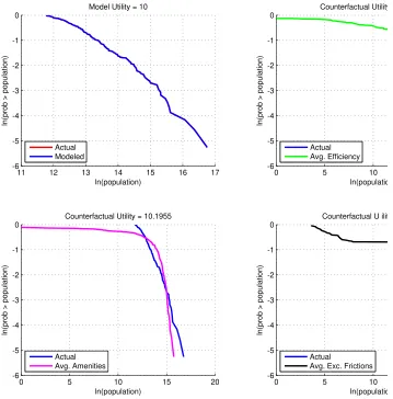
Figure 2 shows three counterfactual exercises where we shut down each of the three shocks (e¢-ciency, amenities, and excessive frictions) respectively. In all cases we eliminate a shock by setting its value to the population weighted average of the shock. We then calculate the utility level that clears the labor market, so total urban population is identical in all cases. Note that eliminating any of the shocks always leads to an increase in utility. Shocks create dispersion in the city size distribution and by equation (8) total commuting costs are convex. So utility in the model tends to increase if population is uniformly distributed in the 192 cities in our sample. If we eliminate all three shocks so that all sites are identical, welfare would increase by3:26%and all cities would have a population of 1 million 68 thousand people. Of course, this increase in welfare does not constitute an upper bound on the importance of the shocks since the distribution of the shocks as well as their correlation matters for the …nal results.

The counterfactual exercises in Figure 2 show that eliminating di¤erences in e¢ciency and ameni-ties has a small e¤ect on utility. In both cases utility would increase by less than 2.5%. The limited e¤ect on utility is due to several reasons. The most obvious one is that population can reallocate across cities. But there are others. For example, the e¤ect of a negative shock to productivity on utility is also mitigated by people working less, by lowering the cost of providing city infrastructure, and by the fact that utility does not only depend on production but also on amenities.

(22)

Appendix A shows …gures and maps with the percentage changes in population for individual cities when we set one of the shocks to its weighted average. In terms of the geographic distribution of city characteristics, we …nd that most cities in the coastal regions would loose population if we eliminated amenity di¤erences. This is consistent with Rappaport and Sachs (2003) who argue that the concentration of population in coastal areas has to do increasingly with a quality of life e¤ect. Central regions would tend to loose population if we eliminated e¢ciency di¤erences as would most of the north-eastern regions. Perhaps the sharpest geographical pattern emerges when we eliminate excessive frictions. Most of the mid-west and north-east (the region that includes the “Rust Belt”) would gain population if we equalize frictions across cities: an indication that governance problems, as well as other labor market frictions, like unions, may be important in these regions.

The e¤ect of the di¤erent shocks on the distribution of city sizes hides some of the implied popu-lation reallocation in these counterfactuals. That is, cities are changing ranking in the distribution even if the overall shape of the distribution does not exhibit large changes, as in the case of excessive frictions. We can calculate reallocation following Davis and Haltiwanger (1992) by adding the num-ber of new workers in expanding cities as a proportion of total population when we change from the actual distribution to the counterfactual. This measure of reallocation is 51.79% when we eliminate di¤erences in TFP, 42.54% when we eliminate amenities, and 9.9% when we eliminate excessive frictions: large numbers given the modest welfare gains. As a benchmark, the same reallocation number for the U.S. economy over a 5 year interval is around 2.1% (2.14% between 2003 and 2008 or 2001 and 2007).

(23)

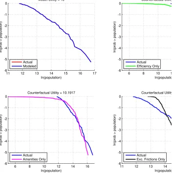
11 12 13 14 15 16 17

Model Utility = 10

Actual

Exc. Frictions Only

Figure 3: Counterfactuals with Only one Shock

The level of commuting costs , which we have estimated to be equal to0:001, is a key parameter in determining the relative importance of each shock. The estimated value implies that agents spend about 2% of their wage income on commuting infrastructure.8 _{The larger , the smaller the relative}

importance of productivity shocks, since it becomes more costly to live in large productive cities and the people that live in them tend to work less since is larger. If we set = 0:005, a …vefold increase, the total reallocation if we equalize e¢ciency across locations drops from around 52% to 10%, with a 1.5% increase in utility, a smaller e¤ect than before. By decreasing the relative importance of productivity shocks, higher transport costs increase the implied dispersion in amenities across cities.

8_{This number seems reasonable: estimates of government spending in transportation infrastructure as a share of}

(24)

As a result, with a …vefold increase in ;reallocations increase from 43% to 45% when cities have average amenities, and utility now goes up by 14.3%, instead of by 2.3%. The reallocation if we set excessive frictions to their average level remains relatively constant at 10%. The changes in city sizes are highly correlated in the exercises with the two di¤erent values of . The correlation in the population changes if we keep amenities constant is 0.53, if we keep e¢ciency constant 0.95, and if we keep excessive frictions constant 0.98.

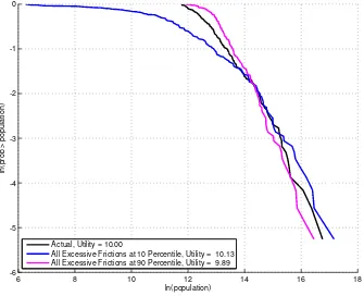
6 8 10 12 14 16 18

-6 -5 -4 -3 -2 -1 0

ln(population)

Actual, Utility = 10.00

All Excessive Frictions at 10 Percentile, Utility = 10.13 All Excessive Frictions at 90 Percentile, Utility = 9.89

Figure 4: Changing the Level of Excessive Frictions

(25)

seen in Section 2.4.

4.1 Adding Production Externalities

So far we have taken productivity in a particular city to be exogenously given. We have assumed that the e¢ciency of a particular site is not a¤ected by the level of economic activity at that site. That is, so far, e¢ciency has explained agglomeration, but we have assumed away the reverse link by which agglomeration explains e¢ciency. Of course, a standard view in urban economics suggests that agglomeration is, at least in part, created by an increase in productivity coming from a rise in the number of people living in a given city. Including these agglomeration e¤ects in our calculations has the potential to change our results, as this will have an endogenous e¤ect on the size of a city.

To incorporate these e¤ects, we start with equation (18) but recognize that the termAit, which captures the e¢ciency of cityi, is a function of the size of the cityNit. In particular, we now let

Ait= ~AitNit!: (20)

That is, the level of productivity is now a function of an exogenous shock Ait~ , and city size, Nit, where the elasticity of the e¢ciency wedge with respect to population is given by !. Note that externalities operate within cities, and not across cities. We can then use the previous calculation of e¢ciency wedges in the data, using equation (2), and divide by population raised to !. The result is a set of new exogenous e¢ciency levels Ait~ . We then substitute (20) in (18) and solve for the it’s that yield the city’s exact population levels. Excessive frictions are calculated as before.

With all the city shocks in hand, we can now perform the same set of counterfactual exercises as before. Note that equation (18) now includesNitin the productivity terms and so cannot be solved analytically. However, we can solve the system of nonlinear equations numerically to obtain city sizes in the counterfactual exercises.

We still need to determine a suitable value for!. Of course, the estimation of equation (14) is not useful to determine !. In fact, this equation will …t exactly as in the data in our simulation of the actual economy. Instead, we rely on the literature, that suggests a fairly robust estimate of!= 0:02

(26)

11 12 13 14 15 16 17

Model Utility = 10

Actual

Counterfactual U ility = 9.9748

Actual

Avg. Exc. Frictions

Figure 5: Counterfactuals Without one Shock and Externalities, = 0:001, != 0:02

(27)

With average e¢ciency, utility declines from 10.25 to 10.12, and for average amenities utility declines from 10.23 to 10.20. The utility levels with average excessive frictions declines from 10.005 to 9.97. The gains are smaller with externalities because even though the convex commuting costs lead to gains if cities become more alike, di¤erences in city characteristics make cities exploit the gains from the external e¤ects. As we increase the elasticity of e¢ciency to population size, the losses from the second channel dominate when we eliminate di¤erences in one of the city characteristics.

Compared to the case without externalities, total reallocation required in the counterfactual tends to go down when we eliminate e¢ciency di¤erences (41.54%). This is natural as now a fraction of the e¢ciency di¤erences is explained by size. For the other two characteristics, reallocation increases slightly to 44.03% in the case of average amenities, and more signi…cantly to 18.46% in the case of average excessive frictions. This happens because the changes introduced by the elimination of these shocks get compounded through the e¤ect of changes in population on e¢ciency.

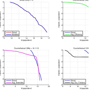
Figure 6 doubles the externality to ! = 0:04: This is closer to the estimate of 0.05 reported by Behrens, Duranton and Robert-Nicoud (2010). In general, the e¤ects discussed before get exacer-bated. Many more cities either exit or become very small. The results suggest that selection of cities in the presence of externalities can be extremely important. Relative to the case without externalities, the increase in externalities lowers the utility gain obtained if we equalize one of the city characteristics. It also increases the decline in utility in the case of average excessive frictions where many cities decline in size substantially. By equalizing exogenous characteristics, some of the more attractive cities no longer bene…t from agglomeration economies, and utility drops.

(28)

11 12 13 14 15 16 17

Model Utility = 10

Actual

Avg. Exc. Frictions

Figure 6: Counterfactuals Without one Shock and Externalities, = 0:001, != 0:04

(29)

4.2 Adding Externalities to Amenities

We can also add externalities in the amenities a city provides. That is, we can let the utility from living in a particular city depend on the size of the city directly. People live in New York because living around a large number of people leads to a scale that provides them with a variety of goods and services, and interactions with people, that they enjoy. We have modeled the preference to live in a particular city through the amenity shocks _it. So we can simply let

it= ~itNit;

where now ~_it is the exogenous amenity shock and is the elasticity of amenities with respect to population size.

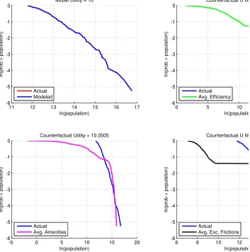
We repeat the exercise in Figure 5 but now we let = 0:02as well. Figure 7 shows the results. The results are qualitatively similar but now we observe that more cities become extremely small. That is, the selection mechanism we emphasized above becomes stronger. Utility in all counterfactuals decreases relative to Figure 5. Including the externality in amenities results now in small losses in the case of identical exogenous productivity across cities, and 0.5% gains in the case where exogenous amenities are constant. The decrease in utility is natural given that with externalities in both production and amenities, equalizing city characteristics implies that externalities are not exploited as much.

(30)

11 12 13 14 15 16 17

Model Utility = 10

Actual

Avg. Exc. Frictions

Figure 7: Counterfactuals Without one Shock and Externalities, = 0:001,!= 0:02, = 0:02

(31)

compute the equilibrium with minimal reallocation of agents across cities, which also yields a level of utility closest to the one in the actual distribution, which we normalize to 10.

6 8 10 12 14 16 18

-6 -5 -4 -3 -2 -1 0

ln(population)

Actual, U ility = 10

No Shocks,  =  = 0.02, Utility = 10.047 No Shocks,  =  = 0.04, Utility = 9 951 No Shocks,  =  = 0.06, Utility = 9 856

Figure 8: Counterfactuals Without Shocks, = 0:001

Figure 8 shows counterfactuals without shocks for di¤erent elasticities of city e¢ciency and ameni-ties to population size. Clearly, as we increase the elasticity, and therefore the externality, we still have two sizes of cities, but the larger the externality, the larger and fewer the larger cities. So larger externalities make the larger and smaller cities larger, and increase the number of small cities. Furthermore, the larger the externality, the lower utility in the counterfactual without shocks. When externalities are large, di¤erences across cities create agglomeration and result in bene…ts. Elimi-nating them yields lower utility.

5. THE EFFECT OF EFFICIENCY AND AMENITY SHOCKS

(32)

factors reallocate in a frictionless manner across cities. There are some dynamics in the process of accumulating capital but we neglect those and focus on the steady state (since these dynamics are just aggregate and have been well studied in the macroeconomics literature).

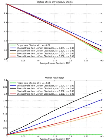
The purpose here is to understand what are the magnitudes of welfare losses if the economy is hit by, say, a 20% negative e¢ciency shock. We consider a proportional decrease in productivity in all cities and a random uniformly distributed proportional shock9 that amounts to di¤erent declines in average productivity. Figure 9 shows the e¤ect on utility (top panel) and worker reallocation (bottom panel). In this exercise we calculate utility including the gains from changes in land rents in order to account exactly for an agent’s welfare (although this has a negligible impact).

As can be seen in Figure 9, if every city experiences a proportional reduction in e¢ciency, the urban hierarchy remains the same, so there is no reallocation of agents. In this case, the value of commuting costs does not a¤ect the slope of the welfare losses: the negative e¤ect on welfare of an increase in the shock is independent of .10 _{The most important observation is that although shocks}

reduce utility, they do so much less than proportionally. The reason is threefold. First, agents can adjust their leisure as a result of the shock as well as the amount of capital. Second, agents obtain utility out of the amenities in the city and so consumption of goods is only one of the elements that determines an agent’s utility. The utility that agents obtain from city amenities amounts, on average, to around 28% of an agent’s utility. Third, commuting costs and the distortions created to build the related public infrastructure go down with productivity and wages.

If cities receive random, but on average negative, TFP shocks, the welfare costs are smaller, since agents can relocate to the cities that received relatively good shocks. For example, for shocks that reduce average TFP by 30%, welfare decreases by 4.6% rather than 5.3%. If we double commuting costs to = 0:002, the overall utility loss is slightly higher, as reallocation tends to go from smaller to larger cities. The impact of higher commuting costs on reallocation is more substantial, since higher congestion costs slow down the move towards larger cities. Overall, random shocks create signi…cantly more reallocation, but the welfare implications are minor. The fact that all curves in the top panel are close to each other suggests that changes in commuting costs, as well as including externalities in production, have small e¤ects on the welfare consequences of these shocks. The …gure also shows that in all these cases the urban structure, and in particular migration between cities,

9_{We use a proportional shock to productivity of the form}_s

it= 0:5 +xit;wherexit U(0;1);andsitis multiplied

by 1 minus the size of the average shock we analyze.

1 0_{Of course, an increase in} _{leads to lower utility as more output is lost on commuting, but this does not show up}

(33)

mitigates the impact of productivity shocks. It is also clear from the graph that the bene…ts from the implied population reallocations are extremely small. In general, adding externalities leads to more reallocation since many cities disappear. However, the welfare impact of these selection e¤ects is, again, very small.

0 0.05 0.1 0.15 0.2 0.25 0.3

9.4 9.5 9.6 9.7 9.8 9.9 10

Average Percent Decline in TFP Welfare Effects of Productivity Shocks

0 0.05 0.1 0.15 0.2 0.25 0.3

0 0.05 0.1 0.15 0.2 0.25 0.3 0.35 0.4

Average Percent Decline in TFP Worker Reallocation Propor ional Shocks, all ,  = 0.00

Shocks Drawn from Uniform Distribution,  = 0.001,  = 0.00 Shocks Drawn from Uniform Distribution,  = 0.001,  = 0.02 Shocks Drawn from Uniform Distribution,  = 0.002,  = 0.00 Shocks Drawn from Uniform Distribution,  = 0.002,  = 0.02

Propor ional Shocks, all ,  = 0.00

Shocks Drawn from Uniform Distribution,  = 0.001,  = 0.00 Shocks Drawn from Uniform Distribution,  = 0.001,  = 0.02 Shocks Drawn from Uniform Distribution,  = 0.002,  = 0.00 Shocks Drawn from Uniform Distribution,  = 0.002,  = 0.02

(34)

0 0.05 0.1 0.15 0.2 0.25 0.3 8.8

9 9.2 9.4 9.6 9.8 10

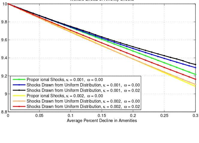
Average Percent Decline in Amenities Welfare Effects of Amenity Shocks

0 0.05 0.1 0.15 0.2 0.25 0.3

0 0.1 0.2 0.3 0.4 0.5

Average Percent Decline in Amenities Worker Reallocation Propor ional Shocks,  = 0.001,  = 0.00

Shocks Drawn from Uniform Distribution,  = 0.001,  = 0.00 Shocks Drawn from Uniform Distribution,  = 0.001,  = 0.02 Propor ional Shocks,  = 0.002,  = 0.00

Shocks Drawn from Uniform Distribution,  = 0.002,  = 0.00 Shocks Drawn from Uniform Distribution,  = 0.002,  = 0.02

Propor ional Shocks,  = 0.001,  = 0.00

Shocks Drawn from Uniform Distribution,  = 0.001,  = 0.00 Shocks Drawn from Uniform Distribution,  = 0.001,  = 0.02 Propor ional Shocks,  = 0.002,  = 0.00

Shocks Drawn from Uniform Distribution,  = 0.002,  = 0.00 Shocks Drawn from Uniform Distribution,  = 0.002,  = 0.02

Figure 10: The E¤ect of Negative Productivity Shocks

(35)

also formed by productivity and the e¤ectiveness in providing urban infrastructure.

The welfare losses from these shocks are larger than in the case of productivity. Since we know that amenities amount to around 28% of average utility, we would expect welfare to go down by slightly more than one quarter of the original shock. The calculation is not exact since reallocation and other adjustments change the actual welfare losses, but it provides a helpful benchmark. In fact, the good accuracy of this back-of-the-envelope calculation shows that the bene…ts from reallocation are again very small. Adding externalities in this case always increases welfare, although not necessarily reallocation (the e¤ect depends on the value of ). In the case of amenity shocks, an increase in the value of has a greater negative e¤ect on welfare, compared to the case of productivity shocks. This happens because amenity shocks imply more reallocation than productivity shocks. The conclusion is that shocks that yield on average a 30% reduction in amenities reduce welfare by around 7%.

6. CHINA

The most important …nding so far is that eliminating di¤erences in e¢ciency, amenities or excessive frictions leads tolarge reallocations of people but tosmall welfare e¤ects. It is unclear whether this conclusion is general, inherent to the model, or speci…c to the U.S. To address this question, we carry out a similar analysis for the case of China.

The details of the database we built for 212 Chinese cities for 2005 are given in Appendix B.2. The data we need are the same as for the U.S. and come from China City Statistics and from the 2005 1% Population Survey. Two further comments are in place. First, in China a prefecture-level city is an administrative division below a province and above a county. Prefecture-level cities cover the entire Chinese geography, and include both the urban parts and the rural hinterlands, and are therefore not the same as cities in the U.S. Luckily, the data tend to provide separate information for the urban parts of cities (referred to as districts under prefecture-level cities or also as city proper). In our database we focus on those districts under prefecture-level cities, as these are the closest equivalents to MSAs in the U.S. Second, when using Chinese data, the issue of their quality inevitably comes up. City level data tend to be collected by local statistical agencies, and are commonly perceived to be of very high quality.11

In order to estimate e¢ciency, amenities and excessive frictions, we need to use parameter values speci…c to the Chinese economy. We set the capital share of income = 0:5221and the real interest

(36)

rater= 0:2008(Bai et al., 2006). Consistent with our analysis of the U.S., we use the same approach as McGrattan and Prescott (2009) to estimate for China and …nd a value of1:5247. Once again, Appendix B.2 provides more details. In any case, the exact values for the di¤erent parameters play a limited role. When using the U.S. parameter values for our exercise on China, the main …ndings are largely unchanged. The reason is that modifying any of the parameter values has a limited impact on the distribution of the relevant variables across cities. We set externalities equal to zero in all exercises with Chinese data.

12 13 14 15 16 17

Model Utility = 10

Counterfactual Utility = 14.6992, Reallocation = 0.64395

Actual

Avg. Exc. Frictions

Figure 11: China Counterfactuals Without one Shock

(37)

excessive frictions). Results for China are shown in Figure 11, and should be compared to the results for the U.S. in Figure 2.12 _{The most striking di¤erence with the U.S. is that the welfare e¤ects in}

China are now an order of magnitude larger. If all Chinese cities had the same level of e¢ciency, welfare would increase by 47%, and if all had the same level of amenities, welfare would increase by 13%. The corresponding …gures for the U.S. are 2.5% and 2.3%.13 _{Another way of seeing the}

di¤erence in magnitude is that in order to maintain utility at its original level, it would be enough to give all Chinese cities an e¢ciency level corresponding to the lowest 27th percentile. Note also that the total reallocation of population is similar to that in the U.S. even though the welfare gains are much larger. Some examples can be informative: Both Beijing and Shanghai would lose about 31% of its population if we equalize productivity. In contrast, if we equalize amenities, Beijing would lose 10% of its population while Shanghai would lose only 1%. Equalizing excessive frictions also leads to large e¤ects in some cities. For example, Shenzhen, one of the “special economic zone” cities would lose 71% of its population if we equalize excessive frictions.

Another di¤erence with the U.S. is that when equalizing e¢ciency or amenities across Chinese cities, the size distribution becomes more dispersed, with the larger cities being larger and the smaller cities being smaller. Large cities in China in general are more e¢cient, but have worse amenities, than smaller cities (in comparison, in the U.S. larger cities score better on both accounts). If all cities had the same amenities, the larger ones would become more attractive, making them even larger. The opposite would happen with the smaller cities. Given that larger cities tend to be more e¢cient, it is not immediately obvious why equalizing e¢ciency levels skews the distribution towards larger cities. What happens here is that some of the intermediate-sized cities, with higher amenities than the largest cities, now get higher levels of e¢ciency, and end up becoming very large cities. In other words, when equalizing amenities, the already larger cities become even larger, whereas when equalizing e¢ciency, some intermediate-sized cities become much larger. This is consistent with population reallocation being lower when equalizing amenities (50%) than when equalizing e¢ciency (64%). Another potential explanation is that large cities, even though they are better at everything, are arti…cially kept small by migration restrictions. The relatively small population combined with large e¢ciency would lead our model to estimate low amenities and high frictions for

1 2_{There is one di¤erence with the exercise we perform for the U.S. When shutting down a shock, we set it equal to}

the median, rather than the weighted mean, of all cities. This change underestimates the di¤erence between China and the U.S. We do this di¤erently because the weighted mean of Chinese city TFP would make cities so productive that an equilibrium with the same number of cities does not exists.

1 3_{Shocks in China were set equal to their median. Given that the median is below the mean, the …gures for China}

(38)

these cities, leading to the mechanism described above. This would be consistent with the …nding of Au and Henderson (2006) that Chinese cities are too small.

We have not yet discussed the e¤ect of equalizing excessive frictions across cities. When setting excessive frictions equal to the median, we …nd that welfare declines by 1.5%. Though much smaller than the e¤ects of amenities and e¢ciency, its e¤ect is, once again, an order of magnitude larger than in the U.S., where the corresponding number is an improvement of 0.05%. The relatively small e¤ect does not imply that excessive frictions are small in China. To see this, Figure 12 shows the impact on welfare and on the city size distribution if excessive frictions are set equal to the 90th and the 10th percentile of the distribution of excessive frictions. If all cities had the excessive frictions of the 90th percentile, welfare would drop by 6%, and the larger cities would become smaller. Likewise, if all cities had the excessive frictions of the 10th percentile, welfare would improve by 4%, and the larger cities would become larger. These e¤ects are substantially larger than the U.S. and far from negligible.

10 11 12 13 14 15 16 17

-6 -5 -4 -3 -2 -1 0

ln(population)

ln(prob > popula

ion)

Excessive Frictions Counterfactuals: China

All Excessive Frictions at 90 Percentile, Utility = 9.3989 All Excessive Frictions at 50 Percentile, Utility = 10 All Excessive Frictions at 10 Percentile, Utility = 10.3834

(39)

7. CONCLUSION

In this paper we have decomposed the size distribution of cities into three main characteristics: e¢ciency, amenities, and excessive frictions. We …nd that each one of these components is important. Eliminating di¤erences in any of them would imply large reallocations of people. In the U.S. the welfare gains or losses associated with particular distributions of these characteristics are very small. Eliminating any di¤erences in characteristics across cities yields welfare gains of at most 3%. Note that the actual population movements required can be larger than 50%, so any small reallocation cost would turn these gains into losses. We also include externalities in both productivity and amenities. The welfare e¤ects associated with eliminating particular characteristics of cities are even smaller in these cases, although we …nd a strong selection e¤ect in the counterfactual distributions. Namely, many cities exit or become extremely small.

The negligible e¤ect in terms of welfare are not inherent to the model. Applying the same method-ology to Chinese cities reveals welfare e¤ects that are an order of magnitude higher. Of course, dynamic models in which reallocation a¤ects the growth rate could also lead to larger changes in welfare in the U.S. The impact on welfare could be further enhanced if one were to add distribu-tional e¤ects in a model with heterogeneous agents, or if the number of cities were smaller, making reallocation by moving to similar cities more di¢cult.

The results for the U.S. also suggest that a potential lack of mobility across locations (that could be caused, for example, by agents being “underwater” with their mortgages) can at most involve limited e¤ects on welfare. We …nd that a 20% reduction in productivity leads to a reduction in welfare of between 3% and 4%, while a reduction of 20% in amenities leads to a reduction in welfare of between 5% and 6%. These reductions in welfare change only by a small fraction of a percent if we use idiosyncratic city shocks that average to the same decline. These results suggest that the implied reallocation of agents that results from idiosyncratic shocks has small welfare e¤ects in the U.S.

(40)

REFERENCES

[1] Albouy, D., 2008. “Are Big Cities Really Bad Places to Live? Improving Quality-of-Life Estimates across Cities,” NBER Working Papers 14472.

[2] Albouy, D., 2009. “What Are Cities Worth? Land Rents, Local Productivity, and the Capitalization of Amenity Values,” NBER Working Papers 14981.

[3] Asdrubali, P., Sorensen, B.E. and Yosha, O., 1996. “Channels of Interstate Risk Sharing: United States 1963-1990,”Quarterly Journal of Economics, 111, 1081-1110.

[4] Au, C.-C. and Henderson, J.V., 2006. “Are Chinese Cities Too Small?”,Review of Economic Studies, 73, 549-576.

[5] Bai, C.-E., Hsieh, C.-T. and Qian, Y., 2006. “The Return to Capital in China,” Brookings Papers on Economic Activity, 37, 61-102.

[6] Behrens, K., Duranton, G. and Robert-Nicoud, F., 2010. “Productive Cities: Sorting, Selection, and Agglomeration,” unpublished manuscript.

[7] Behrens, K., Mion, G., Murata, Y., and Südekum, J., 2010. Agglomeration and Firm Selection, unpublished manuscript.

[8] Bleakley, H. and Lin J., 2010. “Portage: Path Dependence and Increasing Returns in U.S. History,” NBER Working Papers 16314.

[9] Carlino, G., Chatterjee, S., and Hunt, R., 2006. “Urban Density and the Rate of Invention,” Working Paper 06-14, Federal Reserve Bank of Philadelphia.

[10] Chari, V. V., Kehoe, P., McGrattan, E., 2007. “Business Cycle Accounting,” Econometrica, 75, 781-836.

[11] Combes, P, Duranton, G., Gobillon, L., Puga, Diego and Roux, S., 2009. “The productivity ad-vantages of large cities: Distinguishing agglomeration from …rm selection,” CEPR Discussion Papers 7191.

(41)

[13] Córdoba, Juan Carlos, 2008. “On the Distribution of City Sizes,” Journal of Urban Economics, 63, 177-197.

[14] Davis, S.J. and Haltiwanger, J., 1992. “Gross Job Creation, Gross Job Destruction, and Employment Reallocation,”Quarterly Journal of Economics, 107, 819-63.

[15] Davis, D., and Weinstein,D., 2002. “Bones, Bombs, and Break Points: The Geography of Economic Activity,”American Economic Review, 92, 1269-1289.

[16] Duranton, Gilles, 2007. “Urban Evolutions: The Fast, the Slow, and the Still,”American Economic Review, 97, 197-221.

[17] Duranton, Gilles and Henry Overman, 2008. “Exploring the Detailed Location Patterns of U.K. Manufacturing Industries Using Micro-Geographic Data,”Journal of Regional Science, 48, 213-243.

[18] Gabaix, X., 1999a. “Zipf’S Law for Cities: An Explanation,”Quarterly Journal of Economics, 114, 739-767.

[19] Gabaix, X., 1999b. “Zipf’s Law and the Growth of Cities,”American Economic Review, 89, 129-132. [20] Garofalo, G.A. and Yamarik, S., 2002. “Regional Convergence: Evidence from a New State-by-State

Capital Stock Series,”Review of Economics and Statistics,84, 316-323.

[21] Glaeser, E., Kolko, J., and Saiz, A., 2001. “Consumer City,” Journal of Economic Geography, 1, 27-50.

[22] Glaeser, E., Gyourko, J. and Saks, R., 2005. “Why Is Manhattan So Expensive? Regulation and the Rise in Housing Prices,” Journal of Law and Economics, 48, 331-369.

[23] Hess, G.D. and Shin, K., 1997. “International and Intranational Business Cycles,”Oxford Review of Economic Policy, 13, 93-109.

[24] Holmes, T., 2005. “The Location of Sales O¢ces and the Attraction of Cities,”Journal of Political Economy, 113, 551-581.

(42)

[26] Holmes, T., and Stevens, J., 2004. “Spatial distribution of economic activities in North America,”

Handbook of Regional and Urban Economics,in: J. V. Henderson & J. F. Thisse (ed.), V. 4, Chapter 63, 2797-2843, Elsevier.

[27] Lucas, R. E., 1987.Models of Business Cycles, Basil Blackwell.

[28] Lustig, H. and Van Nieuwerburgh, S., 2010. “How Much Does Household Collateral Constrain Regional Risk Sharing?”,Review of Economic Dynamics, 13, 265-294.

[29] McGrattan, E. and Prescott, E., 2009. “Unmeasured Investment and the Puzzling U.S. Boom in the 1990s ,” Research Department Sta¤ Report 369, Federal Reserve Bank of Minneapolis. [30] Rappaport, J., 2008. “Consumption amenities and city population density,” Regional Science and

Urban Economics, 38, 533-552.

[31] Rappaport, J., 2009. “The increasing importance of quality of life,”Journal of Economic Geography, 9, 779-804.

[32] Rappaport, J. and Sachs, J. D., 2003. “The United States as a Coastal Nation,”Journal of Economic Growth, 8, 5-46.

[33] Rossi-Hansberg, Esteban and Mark Wright, 2007. “Urban Structure and Growth,” Review of Eco-nomic Studies, 74, 597-624.